

20
Chapter 2: Misuses
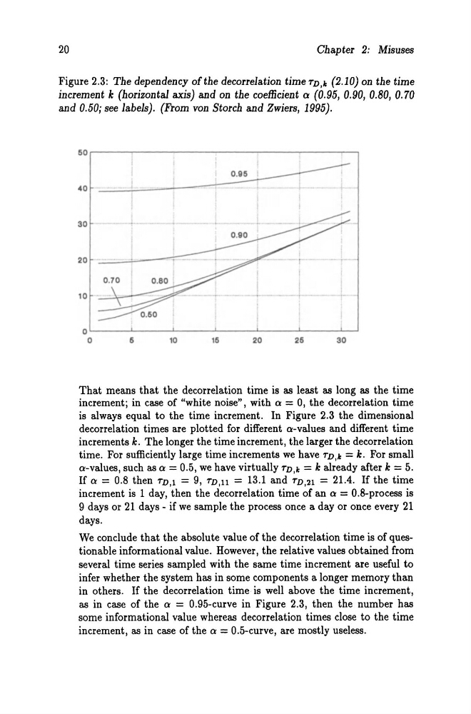
Figure 2.3: The dependency ofthe decorrelation time TD,k (2.10) on the time
increment k (horizontal axis) and on the coefficient a (0.95, 0.90, 0.80, 0.70
and 0.50; see labels). (From von Storch and Zwiers, 1995).
60 .-----~----~------------~------------~_,
40
30
,
.. ~----_... -----'"
20
" -
10
.,. --.-._- ,-- .O ~----~----~------~-----L------~----~-J
o
6
10
16
20
26
30
That means that the decorrelation time is as least as long as the time
incrementj in case of "white noise", with 0 = 0, the decorrelation time
is always equal to the time increment. In Figure 2.3 the dimensional
decorrelation times are plot ted for different a-values and different time
increments k. The longer the time inerement, the larger the deeorrelation
time. For sufliciently large time inerements we have TD,k = k. For small
a-values, such as 0 = 0.5, we have virtually TD,k = k already after k = 5.
If 0 = 0.8 then TD,l = 9, TD,ll = 13.1 and TD,21 = 21.4. If the time
increment is 1 day, then the deeorrelation time of an 0 = 0.8-proeess is
9 days or 21 days - if we sampie the process on ce a day or onee every 21
days.
We eonelude that the absolute value of the deeorrelation time is of questionable information al value. However, the relative values obtained from
several time series sampled with the same time inerement are useful to
infer whether the system has in some eomponents a longer memory than
in others. If the deeorrelation time is weIl above the time inerement,
as in ease of the 0 = 0.95-eurve in Figure 2.3, then the number has
some informational value whereas decorrelation times elose to the time
increment, as in ease of the 0 = 0.5-eurve, are mostly useless.
Chapter 2: Misuses
Figure 2.3: The dependency ofthe decorrelation time TD,k (2.10) on the time
increment k (horizontal axis) and on the coefficient a (0.95, 0.90, 0.80, 0.70
and 0.50; see labels). (From von Storch and Zwiers, 1995).
60 .-----~----~------------~------------~_,
40
30
,
.. ~----_... -----'"
20
" -
10
.,. --.-._- ,-- .O ~----~----~------~-----L------~----~-J
o
6
10
16
20
26
30
That means that the decorrelation time is as least as long as the time
incrementj in case of "white noise", with 0 = 0, the decorrelation time
is always equal to the time increment. In Figure 2.3 the dimensional
decorrelation times are plot ted for different a-values and different time
increments k. The longer the time inerement, the larger the deeorrelation
time. For sufliciently large time inerements we have TD,k = k. For small
a-values, such as 0 = 0.5, we have virtually TD,k = k already after k = 5.
If 0 = 0.8 then TD,l = 9, TD,ll = 13.1 and TD,21 = 21.4. If the time
increment is 1 day, then the deeorrelation time of an 0 = 0.8-proeess is
9 days or 21 days - if we sampie the process on ce a day or onee every 21
days.
We eonelude that the absolute value of the deeorrelation time is of questionable information al value. However, the relative values obtained from
several time series sampled with the same time inerement are useful to
infer whether the system has in some eomponents a longer memory than
in others. If the deeorrelation time is weIl above the time inerement,
as in ease of the 0 = 0.95-eurve in Figure 2.3, then the number has
some informational value whereas decorrelation times elose to the time
increment, as in ease of the 0 = 0.5-eurve, are mostly useless.