

Section 13.3: Empirical Orthogonal Functions
237
(13.17)
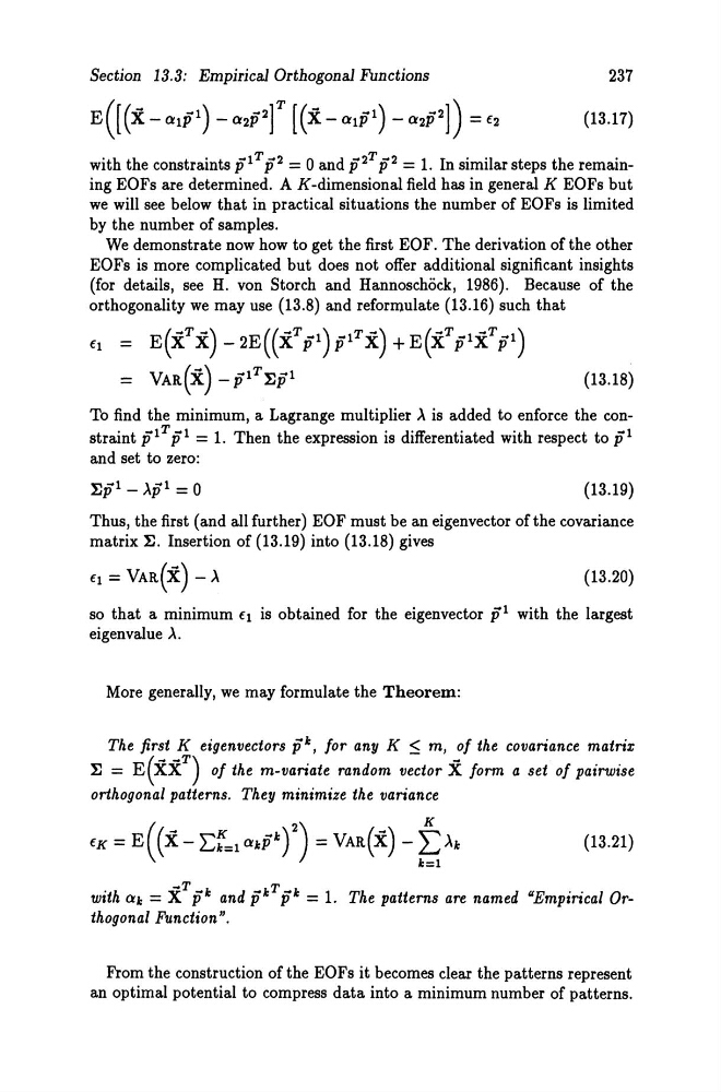
with the constraints plT p2 = 0 and p2 T p2 = 1. In similar steps the remaining EOFs are determined. A K-dimensional field has in general K EOFs but
we will see below that in practical situations the number of EOFs is limited
by the number of sam pIes.
We demonstrate now how to get the first EOF. The derivation of the other
EOFs is more complicated but does not offer additional significant insights
(for details, see H. von Storch and Hannoschöck, 1986). Because of the
orthogonality we may use (13.8) and reformulate (13.16) such that
fl
E(XTX) _2E((X T pl)plTX) +E(XTp1XTpl)
(13.18)
To find the minimum, a Lagrange multiplier A is added to enforce the constraint plT pl = 1. Then the expression is differentiated with respect to pl
and set to zero:
(13.19)
Thus, the first (and all furt her) EOF must be an eigenvector ofthe covariance
matrix lJ. Insertion of (13.19) into (13.18) gives
fl = VAR(X) - A
(13.20)
so that a minimum fl is obtained for the eigenvector pl with the largest
eigenvalue A.
More generally, we may formulate the Theorem:
The first K eigenvectors pk, for any K :::; m, of the covariance matrix
(
~ ~T)
~
lJ = E XX
of the m-variate random vector X form a set of pairwise
orthogonal patterns. They minimize the variance
(13.21 )
with ak = X T pk and pk T pk = 1. The patterns are named "Empirical Orthogonal Funciion".
From the construction of the EOFs it becomes clear the patterns represent
an optimal potential to compress data into a minimum number of patterns.
237
(13.17)
with the constraints plT p2 = 0 and p2 T p2 = 1. In similar steps the remaining EOFs are determined. A K-dimensional field has in general K EOFs but
we will see below that in practical situations the number of EOFs is limited
by the number of sam pIes.
We demonstrate now how to get the first EOF. The derivation of the other
EOFs is more complicated but does not offer additional significant insights
(for details, see H. von Storch and Hannoschöck, 1986). Because of the
orthogonality we may use (13.8) and reformulate (13.16) such that
fl
E(XTX) _2E((X T pl)plTX) +E(XTp1XTpl)
(13.18)
To find the minimum, a Lagrange multiplier A is added to enforce the constraint plT pl = 1. Then the expression is differentiated with respect to pl
and set to zero:
(13.19)
Thus, the first (and all furt her) EOF must be an eigenvector ofthe covariance
matrix lJ. Insertion of (13.19) into (13.18) gives
fl = VAR(X) - A
(13.20)
so that a minimum fl is obtained for the eigenvector pl with the largest
eigenvalue A.
More generally, we may formulate the Theorem:
The first K eigenvectors pk, for any K :::; m, of the covariance matrix
(
~ ~T)
~
lJ = E XX
of the m-variate random vector X form a set of pairwise
orthogonal patterns. They minimize the variance
(13.21 )
with ak = X T pk and pk T pk = 1. The patterns are named "Empirical Orthogonal Funciion".
From the construction of the EOFs it becomes clear the patterns represent
an optimal potential to compress data into a minimum number of patterns.