

230
Chapter 13: Spatial Patterns: EOFs and CCA
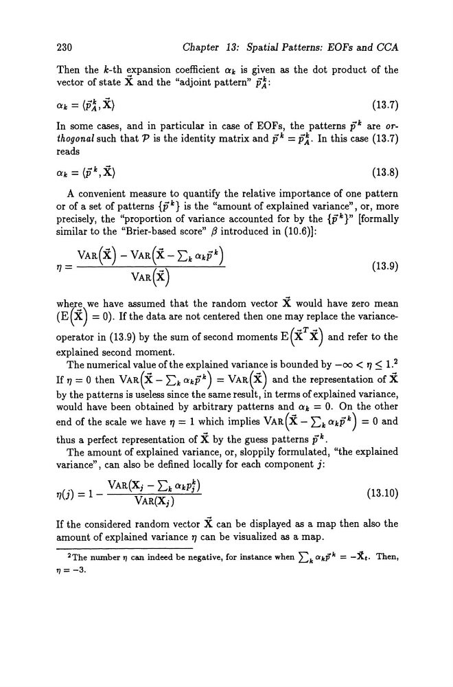
Then the k-th expansion coefficient Qk is given as the dot product of the
vector of state X and the "adjoint pattern" p~:
(13.7)
In some cases, and in particular in case of EOFs, the patterns pk are orthogonal such that P is the identity matrix and pk = p!. In this case (13.7)
reads
(13.8)
A convenient measure to quantify the relative importance of one pattern
or of a set of patterns {p k} is the "amount of explained variance" , or, more
precisely, the "proportion of variance accounted for by the {pk}" [formally
similar to the "Brier-based score" ß introduced in (10.6)]:
(13.9)
wh7:e we have assumed that the random vector X would have zero mean
(E ~ X) = 0). If the data are not centered then one may replace the variance( ~T ~)
operator in (13.9) by the sum of second moments E X X and refer to the
explained second moment.
The numerical value ofthe explained variance is bounded by -00 < TJ ::; 1. 2
If 1] = 0 then VAR(X - Lk OIkpk) = VAR(X) and the representation of X
by the patterns is useless since the same result, in terms of explained variance,
would have been obtained by arbitrary patterns and Qk = O. On the other
end of the scale we have TJ = 1 which implies VAR(X - Ek OIkpk) = 0 and
thus aperfect representation of X by the guess patterns pk.
The amount of explained variance, or, sloppily formulated, "the explained
variance", can also be defined locally for each component j:
(13.10)
If the considered random vector X can be displayed as a map then also the
amount of explained variance 7J can be visualized as a map.
2The number TI can indeed be negative, Cor instance when Ek Otkpk = -Xt. Then,
TI = -3.
Chapter 13: Spatial Patterns: EOFs and CCA
Then the k-th expansion coefficient Qk is given as the dot product of the
vector of state X and the "adjoint pattern" p~:
(13.7)
In some cases, and in particular in case of EOFs, the patterns pk are orthogonal such that P is the identity matrix and pk = p!. In this case (13.7)
reads
(13.8)
A convenient measure to quantify the relative importance of one pattern
or of a set of patterns {p k} is the "amount of explained variance" , or, more
precisely, the "proportion of variance accounted for by the {pk}" [formally
similar to the "Brier-based score" ß introduced in (10.6)]:
(13.9)
wh7:e we have assumed that the random vector X would have zero mean
(E ~ X) = 0). If the data are not centered then one may replace the variance( ~T ~)
operator in (13.9) by the sum of second moments E X X and refer to the
explained second moment.
The numerical value ofthe explained variance is bounded by -00 < TJ ::; 1. 2
If 1] = 0 then VAR(X - Lk OIkpk) = VAR(X) and the representation of X
by the patterns is useless since the same result, in terms of explained variance,
would have been obtained by arbitrary patterns and Qk = O. On the other
end of the scale we have TJ = 1 which implies VAR(X - Ek OIkpk) = 0 and
thus aperfect representation of X by the guess patterns pk.
The amount of explained variance, or, sloppily formulated, "the explained
variance", can also be defined locally for each component j:
(13.10)
If the considered random vector X can be displayed as a map then also the
amount of explained variance 7J can be visualized as a map.
2The number TI can indeed be negative, Cor instance when Ek Otkpk = -Xt. Then,
TI = -3.