

192
Chapter 10: The Evaluation of Forecasts
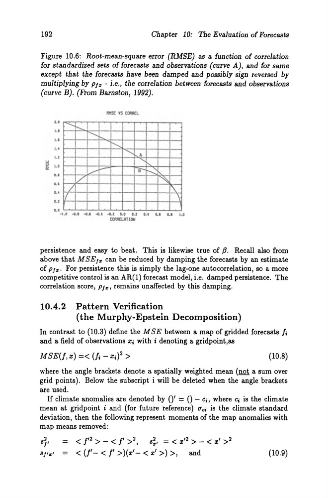
Figure 10.6: Root-mean-square error (RMSE) as a function of correlation
for standardized sets of forecasts and observations (curve A), and for same
except that the forecasts have been damped and possibly sign reversed by
multiplying by Piz - i.e., the correlation between forecasts and observations
(curve B). (From Barnston, 1992).
I.'
1.'
I.'
.......... I"--...
j""--..",
1.'
1.1
~ \.'
0.'
0.'
I.'
O.Z
I"---..
........... A
"i',.
,....... I--"
B- r---..::
/'
~
/
I\.
11
\
...
-1.' ~.I ~.I ~. -o.z 1.1 LI 1.1 LI 1.1 1.0
aJRRWIT IIJI
persistence and easy to beat. This is likewise true of ß. Recall also from
above that MSElz can be reduced by damping the forecasts by an estimate
of Piz' For persistence this is simply the lag-one autocorrelation, so a more
competitive control is an AR(!) fore cast model, i.e. damped persistence. The
correlation score, Piz, remains unaffected by this damping.
10.4.2 Pattern Verification
(the Murphy-Epstein Decomposition)
In contrast to (10.3) define the M SE between a map of gridded forecasts fi
and a field of observations Xi with i denoting a gridpoint,as
(10.8)
where the angle brackets denote a spatially weighted mean (not a sum over
grid points). Below the subscript i will be deleted when the angle brackets
are used.
If climate anomalies are denoted by 0' = 0 - Ci, where Ci is the climate
mean at gridpoint i and (for future reference) Uoi is the climate standard
deviation, then the following represent moments of the map anomalies with
map means removed:
< 1'2 > - < I' >2, S~' = < X /2 > _ < X' >2
< (1'- < I' »(x ' - < X' » >, and
(10.9)
Chapter 10: The Evaluation of Forecasts
Figure 10.6: Root-mean-square error (RMSE) as a function of correlation
for standardized sets of forecasts and observations (curve A), and for same
except that the forecasts have been damped and possibly sign reversed by
multiplying by Piz - i.e., the correlation between forecasts and observations
(curve B). (From Barnston, 1992).
I.'
1.'
I.'
.......... I"--...
j""--..",
1.'
1.1
~ \.'
0.'
0.'
I.'
O.Z
I"---..
........... A
"i',.
,....... I--"
B- r---..::
/'
~
/
I\.
11
\
...
-1.' ~.I ~.I ~. -o.z 1.1 LI 1.1 LI 1.1 1.0
aJRRWIT IIJI
persistence and easy to beat. This is likewise true of ß. Recall also from
above that MSElz can be reduced by damping the forecasts by an estimate
of Piz' For persistence this is simply the lag-one autocorrelation, so a more
competitive control is an AR(!) fore cast model, i.e. damped persistence. The
correlation score, Piz, remains unaffected by this damping.
10.4.2 Pattern Verification
(the Murphy-Epstein Decomposition)
In contrast to (10.3) define the M SE between a map of gridded forecasts fi
and a field of observations Xi with i denoting a gridpoint,as
(10.8)
where the angle brackets denote a spatially weighted mean (not a sum over
grid points). Below the subscript i will be deleted when the angle brackets
are used.
If climate anomalies are denoted by 0' = 0 - Ci, where Ci is the climate
mean at gridpoint i and (for future reference) Uoi is the climate standard
deviation, then the following represent moments of the map anomalies with
map means removed:
< 1'2 > - < I' >2, S~' = < X /2 > _ < X' >2
< (1'- < I' »(x ' - < X' » >, and
(10.9)