

Section 9.2: Motivation
165
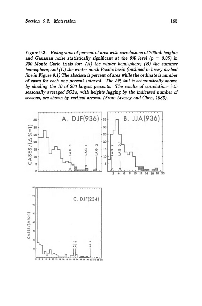
Figure 9.3: Histograms of percent of area with correlations of 700mb heights
and Gaussian noise statistically significant at the 5% level (p = 0.05) in
200 Monte Carlo trials for: (A) the winter hemispherej (E) the summer
hemispherej and (C) the winter north Pacific basin (outlined in heavy dashed
line in Figure 9.1) The abscissa is percent ofarea while the ordinate is number
of cases for each one percent interval. The 5% tail is schematically shown
by shading the 10 of 200 largest percents. The results of correlations i-th
seasonally averaged SOl's, with heights lagging by the indicated number of
seasons, are shown by vertical arrows. (From Livezey and Chen, 1983).
35
-:::-30
11
~25
~30
..........
\I) IS
w
\I)
«
10
u 11
n
'0
10
- . .
'ii
~
11)
w :10
11)
«
u
HI
A. DJF(936) 35
B. JJA(936)
30
25
20
...
Cl
Cl
15 Cl
«
«
<
-'
-'
10
...
11
C. DJF(234)
165
Figure 9.3: Histograms of percent of area with correlations of 700mb heights
and Gaussian noise statistically significant at the 5% level (p = 0.05) in
200 Monte Carlo trials for: (A) the winter hemispherej (E) the summer
hemispherej and (C) the winter north Pacific basin (outlined in heavy dashed
line in Figure 9.1) The abscissa is percent ofarea while the ordinate is number
of cases for each one percent interval. The 5% tail is schematically shown
by shading the 10 of 200 largest percents. The results of correlations i-th
seasonally averaged SOl's, with heights lagging by the indicated number of
seasons, are shown by vertical arrows. (From Livezey and Chen, 1983).
35
-:::-30
11
~25
~30
..........
\I) IS
w
\I)
«
10
u 11
n
'0
10
- . .
'ii
~
11)
w :10
11)
«
u
HI
A. DJF(936) 35
B. JJA(936)
30
25
20
...
Cl
Cl
15 Cl
«
«
<
-'
-'
10
...
11
C. DJF(234)