

Section 5.6: Quantifying Climate Signals
91
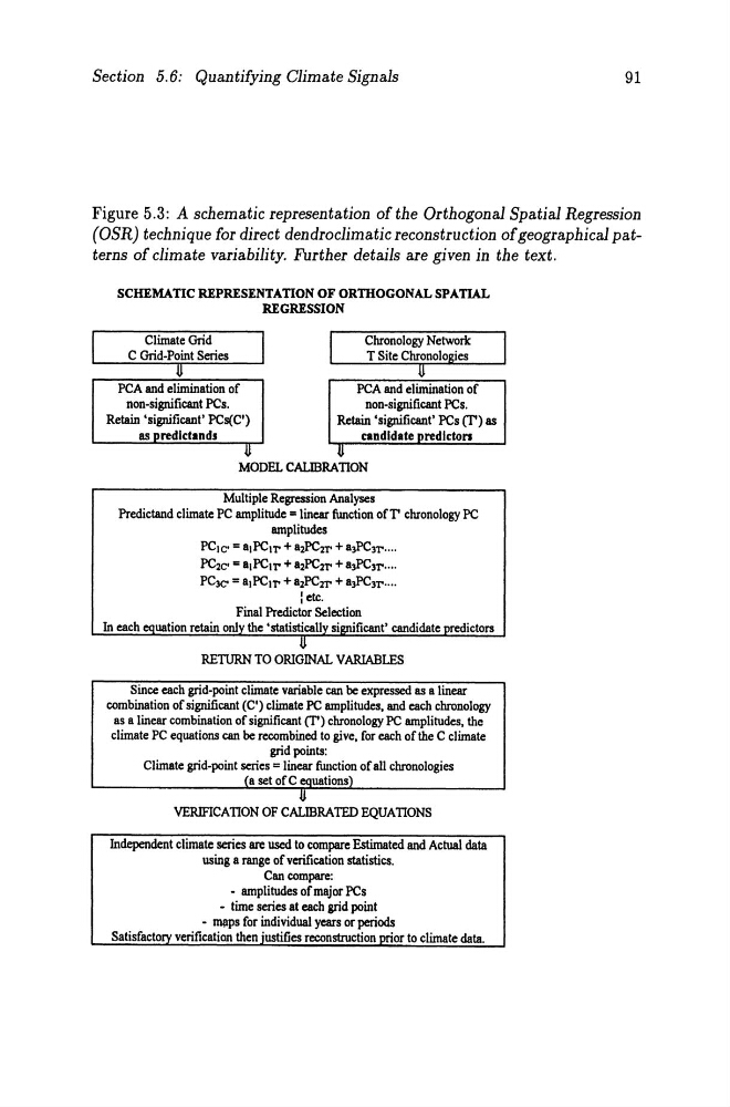
Figure 5.3: A schematic representation of the Orthogonal Spatial Regression
(OSR) technique for direct den droclim atic reconstruction of geographical patterns of climate variability. Further details are given in the text.
SCHEMATIC REPRESENTATION OF ORTHOGONAL SPATIAL
REGRESSION
Climate Grid
C Grid-Point Series
PCA and elimination of
non-significant PCs.
Retain 'significant' PCs(C'}
as predlctands
U
PCA and elimination of
non-significant PCs.
Retain 'significant' PCs (T') as
tandldate redlcton
MODEL CALIBRATION
Multiple Regression Analyses
Predictand climate PC amplitude = linear function ofT' chronology PC
amplitudes
PCte· = alPCIT' + a2PC2T' + a~C3T' ....
PC2C' = alPCtT' + a2PC2T' + a3PC3T'''''
PC3C' = alPCtT' + a2PC2T' + a3PC3T'''''
: etc.
Final Predictor Selection
In each equation retain only the 'statistically significant' candidate predictors
1.1
RETURN TO ORIGINAL VARIABLES
Since each grid-point climate variable can be expressed as a linear
combination of significant (C') climate PC amplitudes, and each chronology
as a linear combination of significant (T') chronology PC amplitudes, the
climate PC equations can be recombined to give, for each ofthe C climate
grid points:
Climate grid-point series = linear function of all chronologies
(a set ofC equations)
U
VERIFICATION OF CALmRATED EQUATIONS
Independent c1imate series are used to compare Estimated and ActuaI data
using a range of verification statisties.
Can compare:
- amplitudes ofmajor PCs
- time series at each grid point
- mllps for individual years or perlods
Satisfactory verification then justifies reconstruction prior to climate data.
91
Figure 5.3: A schematic representation of the Orthogonal Spatial Regression
(OSR) technique for direct den droclim atic reconstruction of geographical patterns of climate variability. Further details are given in the text.
SCHEMATIC REPRESENTATION OF ORTHOGONAL SPATIAL
REGRESSION
Climate Grid
C Grid-Point Series
PCA and elimination of
non-significant PCs.
Retain 'significant' PCs(C'}
as predlctands
U
PCA and elimination of
non-significant PCs.
Retain 'significant' PCs (T') as
tandldate redlcton
MODEL CALIBRATION
Multiple Regression Analyses
Predictand climate PC amplitude = linear function ofT' chronology PC
amplitudes
PCte· = alPCIT' + a2PC2T' + a~C3T' ....
PC2C' = alPCtT' + a2PC2T' + a3PC3T'''''
PC3C' = alPCtT' + a2PC2T' + a3PC3T'''''
: etc.
Final Predictor Selection
In each equation retain only the 'statistically significant' candidate predictors
1.1
RETURN TO ORIGINAL VARIABLES
Since each grid-point climate variable can be expressed as a linear
combination of significant (C') climate PC amplitudes, and each chronology
as a linear combination of significant (T') chronology PC amplitudes, the
climate PC equations can be recombined to give, for each ofthe C climate
grid points:
Climate grid-point series = linear function of all chronologies
(a set ofC equations)
U
VERIFICATION OF CALmRATED EQUATIONS
Independent c1imate series are used to compare Estimated and ActuaI data
using a range of verification statisties.
Can compare:
- amplitudes ofmajor PCs
- time series at each grid point
- mllps for individual years or perlods
Satisfactory verification then justifies reconstruction prior to climate data.