

Introduction to Numerical Weather Prediction Data Assimilation
91
satisfy, to acceptable accuracy for meteorological order of magnitude of the estimation error,
the relations
M(ti, to)(x(to) + ox(to))
M(ti, to)x(to) + R(ti' to)ox(tO)
Hi(x(ti) + ox(t;)) ::e Hix(t;J + H' ·OX(ti)
( 4.17)
for perturbation ox( to), then the 4D-Var problem P4D is equivalent to the so-called extended
Kalman filter under the above-mentioned hypothesis, namely the quasi-linearity, the perfect
model and the fixed lag (see previous references). This consists of two steps ( f and a denote
forecast and analysis respectively).
4D-Var implicitly uses flow-dependent structure functions as can be seen from equation (4.12)
(Thepaut et ai., 1993a), so that 4D-Var is a scientific improvement on the current operational
implementation. Moreover, 4D-Var is also an algorithmic improvement on the Kalman filter
(4.11-4.15) where the equation (4.12) has to be solved explicitly, instead of implicitly in 4D- Var.
There are two main weaknesses in the 4D- Var implementation. First, the model is assumed to be
perfect: in Eq. (4.12) no source terms Q are present (Talagrand, 1988; Cohn and Parrish, 1991;
Daley, 1991; Wergen, 1992), nevertheless Derber (1989) and Zupanski (1993) demonstrated
how to address a model bias in 4D-Var. Second, we do not have access to the analysis error
covariance Ba(tN) . Here we suggest that, if (4.12) is approximate anyway, it is not scientifically
worthwhile solving it exactly. This idea has been followed by most of the NWP centres which
implemented optimal interpolation; the dynamics R was replaced by the identity or a simple law
for the temporal evolution of the variances. In the Kalman filter context, this is discussed e.g.
by Dee (1991) and Cohn (1992). In other words, it may be scientifically acceptable to replace
R by an approximate tangent-linear model in (4.2) provided this approximation is smaller than
the approximation of neglecting the model error source term Q.
4.4.3 The incremental formulation of variational assimilation
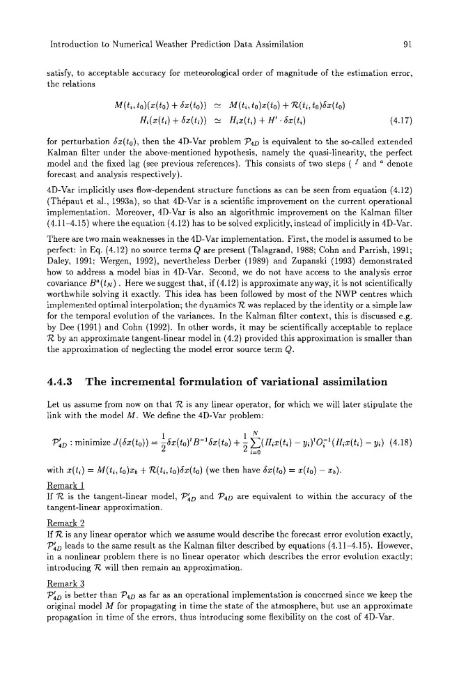
Let us assume from now on that R is any linear operator, for which we will later stipulate the
link with the model M. We define the 4D-Var problem:
with X(ti) = M(ti, to)Xb + R(ti, to)ox(to) (we then have ox(to) = x(to) - Xb).
Remark 1
If R is the tangent-linear model, P~D and P4 D are equivalent to within the accuracy of the
tangent-linear approximation.
Remark 2
If R is any linear operator which we assume would describe the forecast error evolution exactly,
P~D leads to the same result as the Kalman filter described by equations (4.11-4.15). However,
in a nonlinear problem there is no linear operator which describes the error evolution exactly;
introducing R will then remain an approximation.
Remark 3
P~D is better than P4D as far as an operational implementation is concerned since we keep the
original model M for propagating in time the state of the atmosphere, but use an approximate
propagation in time of the errors, thus introducing some flexibility on the cost of 4D-Var.
91
satisfy, to acceptable accuracy for meteorological order of magnitude of the estimation error,
the relations
M(ti, to)(x(to) + ox(to))
M(ti, to)x(to) + R(ti' to)ox(tO)
Hi(x(ti) + ox(t;)) ::e Hix(t;J + H' ·OX(ti)
( 4.17)
for perturbation ox( to), then the 4D-Var problem P4D is equivalent to the so-called extended
Kalman filter under the above-mentioned hypothesis, namely the quasi-linearity, the perfect
model and the fixed lag (see previous references). This consists of two steps ( f and a denote
forecast and analysis respectively).
4D-Var implicitly uses flow-dependent structure functions as can be seen from equation (4.12)
(Thepaut et ai., 1993a), so that 4D-Var is a scientific improvement on the current operational
implementation. Moreover, 4D-Var is also an algorithmic improvement on the Kalman filter
(4.11-4.15) where the equation (4.12) has to be solved explicitly, instead of implicitly in 4D- Var.
There are two main weaknesses in the 4D- Var implementation. First, the model is assumed to be
perfect: in Eq. (4.12) no source terms Q are present (Talagrand, 1988; Cohn and Parrish, 1991;
Daley, 1991; Wergen, 1992), nevertheless Derber (1989) and Zupanski (1993) demonstrated
how to address a model bias in 4D-Var. Second, we do not have access to the analysis error
covariance Ba(tN) . Here we suggest that, if (4.12) is approximate anyway, it is not scientifically
worthwhile solving it exactly. This idea has been followed by most of the NWP centres which
implemented optimal interpolation; the dynamics R was replaced by the identity or a simple law
for the temporal evolution of the variances. In the Kalman filter context, this is discussed e.g.
by Dee (1991) and Cohn (1992). In other words, it may be scientifically acceptable to replace
R by an approximate tangent-linear model in (4.2) provided this approximation is smaller than
the approximation of neglecting the model error source term Q.
4.4.3 The incremental formulation of variational assimilation
Let us assume from now on that R is any linear operator, for which we will later stipulate the
link with the model M. We define the 4D-Var problem:
with X(ti) = M(ti, to)Xb + R(ti, to)ox(to) (we then have ox(to) = x(to) - Xb).
Remark 1
If R is the tangent-linear model, P~D and P4 D are equivalent to within the accuracy of the
tangent-linear approximation.
Remark 2
If R is any linear operator which we assume would describe the forecast error evolution exactly,
P~D leads to the same result as the Kalman filter described by equations (4.11-4.15). However,
in a nonlinear problem there is no linear operator which describes the error evolution exactly;
introducing R will then remain an approximation.
Remark 3
P~D is better than P4D as far as an operational implementation is concerned since we keep the
original model M for propagating in time the state of the atmosphere, but use an approximate
propagation in time of the errors, thus introducing some flexibility on the cost of 4D-Var.