

76
J.D. Albertson, G. Kiely and M.B. Parlange
DSl
DCSl
FCSl
3 Sub layer Model
10 1
Produellon
Olsslpallon (We71)
w
e
100 ,
1\,1,,'11. 1,, '1:;';;':": ':"::'':': :"'::::':: '
~~~--if---r
10.1 ~~~~~U-~~~~wu~~~~~~~~~~~
1~
1~
1~
1~
101
-z/l
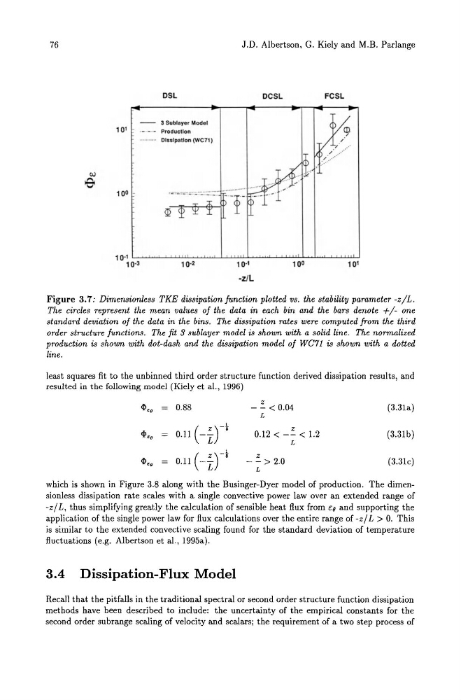
Figure 3.7: Dimensionless TKE dissipation function plotted vs. the stability parameter -zIL.
The circles represent the mean values of the data in each bin and the bars denote +1- one
standard deviation of the data in the bins. The dissipation rates were computed from the third
order structure functions. The fit 3 sublayer model is shown with a solid line. The normalized
production is shown with dot-dash and the dissipation model of we7l is shown with a dotted
line.
least squares fit to the unbinned third order structure function derived dissipation results, and
resulted in the following model (Kiely et al., 1996)
cI> ••
0.88
- -=- < 0.04
(3.31a)
L
cI> ••
0.11 ( _±)-t 0.12 < --=- < 1.2
(3.31 b)
L
cI> •• = 0.11 ( _±)-k - -=- > 2.0
(3.31c)
L
which is shown in Figure 3.8 along with the Businger-Dyer model of production. The dimensionless dissipation rate scales with a single convective power law over an extended range of
-z/ L, thus simplifying greatly the calculation of sensible heat flux from to and supporting the
application of the single power law for flux calculations over the entire range of -z/ L > O. This
is similar to the extended convective scaling found for the standard deviation of temperature
fluctuations (e.g. Albertson et al., 1995a).
3.4 Dissipation-Flux Model
Recall that the pitfalls in the traditional spectral or second order structure function dissipation
methods have been described to include: the uncertainty of the empirical constants for the
second order subrange scaling of velocity and scalars; the requirement of a two step process of
J.D. Albertson, G. Kiely and M.B. Parlange
DSl
DCSl
FCSl
3 Sub layer Model
10 1
Produellon
Olsslpallon (We71)
w
e
100 ,
1\,1,,'11. 1,, '1:;';;':": ':"::'':': :"'::::':: '
~~~--if---r
10.1 ~~~~~U-~~~~wu~~~~~~~~~~~
1~
1~
1~
1~
101
-z/l
Figure 3.7: Dimensionless TKE dissipation function plotted vs. the stability parameter -zIL.
The circles represent the mean values of the data in each bin and the bars denote +1- one
standard deviation of the data in the bins. The dissipation rates were computed from the third
order structure functions. The fit 3 sublayer model is shown with a solid line. The normalized
production is shown with dot-dash and the dissipation model of we7l is shown with a dotted
line.
least squares fit to the unbinned third order structure function derived dissipation results, and
resulted in the following model (Kiely et al., 1996)
cI> ••
0.88
- -=- < 0.04
(3.31a)
L
cI> ••
0.11 ( _±)-t 0.12 < --=- < 1.2
(3.31 b)
L
cI> •• = 0.11 ( _±)-k - -=- > 2.0
(3.31c)
L
which is shown in Figure 3.8 along with the Businger-Dyer model of production. The dimensionless dissipation rate scales with a single convective power law over an extended range of
-z/ L, thus simplifying greatly the calculation of sensible heat flux from to and supporting the
application of the single power law for flux calculations over the entire range of -z/ L > O. This
is similar to the extended convective scaling found for the standard deviation of temperature
fluctuations (e.g. Albertson et al., 1995a).
3.4 Dissipation-Flux Model
Recall that the pitfalls in the traditional spectral or second order structure function dissipation
methods have been described to include: the uncertainty of the empirical constants for the
second order subrange scaling of velocity and scalars; the requirement of a two step process of