

Satellite Remote Sensing of Evaporation over Sea
447
1.0
-Q [W/m2]
0.8
700
600
gO.6
500
~
400
0.2
200
100
0.0
r8
0
2
3
u. [cm/s]
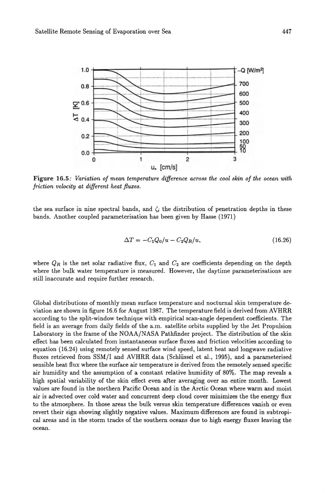
Figure 16.5: Variation of mean temperature difference across the cool skin of the ocean with
friction velocity at different heat fluxes .
the sea surface in nine spectral bands, and (i the distribution of penetration depths in these
bands. Another coupled parameterisation has been given by Hasse (1971)
(16.26)
where QR is the net solar radiative flux, C1 and C2 are coefficients depending on the depth
where the bulk water temperature is measured. However, the daytime parameterisations are
still inaccurate and require further research.
Global distributions of monthly mean surface temperature and nocturnal skin temperature deviation are shown in figure 16.6 for August 1987. The temperature field is derived from AVHRR
according to the split-window technique with empirical scan-angle dependent coefficients. The
field is an average from daily fields of the a.m. satellite orbits supplied by the Jet Propulsion
Laboratory in the frame of the NOAA/NASA Pathfinder project. The distribution of the skin
effect has been calculated from instantaneous surface fluxes and friction velocities according to
equation (16.24) using remotely sensed surface wind speed, latent heat and longwave radiative
fluxes retrieved from SSM/I and AVHRR data (Schliissel et al., 1995), and a parameterised
sensible heat flux where the surface air temperature is derived from the remotely sensed specific
air humidity and the assumption of a constant relative humidity of 80%. The map reveals a
high spatial variability of the skin effect even after averaging over an entire month. Lowest
values are found in the northern Pacific Ocean and in the Arctic Ocean where warm and moist
air is advected over cold water and concurrent deep cloud cover minimizes the the energy flux
to the atmosphere. In those areas the bulk versus skin temperature differences vanish or even
revert their sign showing slightly negative values. Maximum differences are found in subtropical areas and in the storm tracks of the southern oceans due to high energy fluxes leaving the
ocean.
447
1.0
-Q [W/m2]
0.8
700
600
gO.6
500
~
400
0.2
200
100
0.0
r8
0
2
3
u. [cm/s]
Figure 16.5: Variation of mean temperature difference across the cool skin of the ocean with
friction velocity at different heat fluxes .
the sea surface in nine spectral bands, and (i the distribution of penetration depths in these
bands. Another coupled parameterisation has been given by Hasse (1971)
(16.26)
where QR is the net solar radiative flux, C1 and C2 are coefficients depending on the depth
where the bulk water temperature is measured. However, the daytime parameterisations are
still inaccurate and require further research.
Global distributions of monthly mean surface temperature and nocturnal skin temperature deviation are shown in figure 16.6 for August 1987. The temperature field is derived from AVHRR
according to the split-window technique with empirical scan-angle dependent coefficients. The
field is an average from daily fields of the a.m. satellite orbits supplied by the Jet Propulsion
Laboratory in the frame of the NOAA/NASA Pathfinder project. The distribution of the skin
effect has been calculated from instantaneous surface fluxes and friction velocities according to
equation (16.24) using remotely sensed surface wind speed, latent heat and longwave radiative
fluxes retrieved from SSM/I and AVHRR data (Schliissel et al., 1995), and a parameterised
sensible heat flux where the surface air temperature is derived from the remotely sensed specific
air humidity and the assumption of a constant relative humidity of 80%. The map reveals a
high spatial variability of the skin effect even after averaging over an entire month. Lowest
values are found in the northern Pacific Ocean and in the Arctic Ocean where warm and moist
air is advected over cold water and concurrent deep cloud cover minimizes the the energy flux
to the atmosphere. In those areas the bulk versus skin temperature differences vanish or even
revert their sign showing slightly negative values. Maximum differences are found in subtropical areas and in the storm tracks of the southern oceans due to high energy fluxes leaving the
ocean.