

32
A.D. Del Genio
2.3 discusses several physics-based approaches to the question of predicting regional aspects of
climate change. Section 2.4 then outlines a multi-tiered observational strategy for the eventual
accurate modeling of climate change based on validation, physical process, and monitoring
components. Section 2.5 concludes with some thoughts on the future assessment of whether
climate models are good enough for their intended applications.
2.2 Myths and Methods of Climate Model Diagnosis
Satellite data sets currently in existence provide good integrated measures of several important
climate parameters such as top-of-the-atmosphere (TOA) shortwave and long wave radiation
fluxes, total cloud cover, and vertically integrated precipitable water vapor. These serve in
principle as zeroth order validation tools for climate GCMs. It is possible with appropriate
selection of free parameters in climate model parameterizations to match the globally integrated
values of such quantities as well as some features of their geographical distributions, but this by
itself tells us nothing about the utility of the models for predicting climate change. Evidence
of the degree of tuning inherent in climate models is provided by their wildly varying estimates
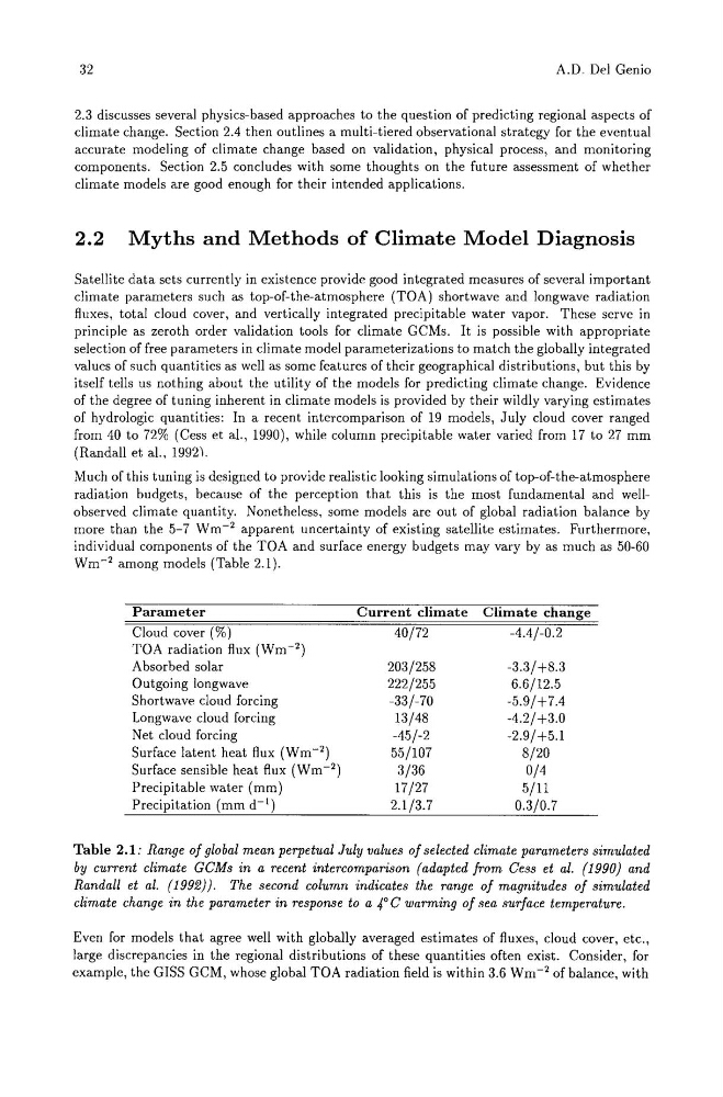
of hydrologic quantities: In a recent intercomparison of 19 models, July cloud cover ranged
from 40 to 72% (Cess et al., 1990), while column precipitable water varied from 17 to 27 mm
(Randall et al., 1992).
Much of this tuning is designed to provide realistic looking simulations of top-of-the-atmosphere
radiation budgets, because of the perception that this is the most fundamental and wellobserved climate quantity. Nonetheless, some models are out of global radiation balance by
more than the 5-7 Wm- 2 apparent uncertainty of existing satellite estimates. Furthermore,
individual components of the TOA and surface energy budgets may vary by as much as 50-60
Wm- 2 among models (Table 2.1).
Parameter
Cloud cover (%)
TOA radiation flux (Wm-2)
Absorbed solar
Outgoing longwave
Shortwave cloud forcing
Longwave cloud forcing
Net cloud forcing
Surface latent heat flux (Wm-2)
Surface sensible heat flux (Wm-2)
Precipitable water (mm)
Precipitation (mm d- 1 )
Current climate
40/72
203/258
222/255
-33/-70
13/48
-45/-2
55/107
3/36
17/27
2.1/3.7
Climate change
-4.4/-0.2
-3.3/ +8.3
6.6/12.5
-5.9/+7.4
-4.2/+3.0
-2.9/+5.1
8/20
0/4
5/11
0.3/0.7
Table 2.1: Range of global mean perpetual July values of selected climate parameters simulated
by current climate GCMs in a recent intercomparison (adapted from Cess et al. (1990) and
Randall et al. (1992)). The second column indicates the range of magnitudes of simulated
climate change in the parameter in response to a 4°C warming of sea surface temperature.
Even for models that agree well with globally averaged estimates of fluxes, cloud cover, etc.,
large discrepancies in the regional distributions of these quantities often exist. Consider, for
example, the GISS GCM, whose global TOA radiation field is within 3.6 Wm- 2 of balance, with
A.D. Del Genio
2.3 discusses several physics-based approaches to the question of predicting regional aspects of
climate change. Section 2.4 then outlines a multi-tiered observational strategy for the eventual
accurate modeling of climate change based on validation, physical process, and monitoring
components. Section 2.5 concludes with some thoughts on the future assessment of whether
climate models are good enough for their intended applications.
2.2 Myths and Methods of Climate Model Diagnosis
Satellite data sets currently in existence provide good integrated measures of several important
climate parameters such as top-of-the-atmosphere (TOA) shortwave and long wave radiation
fluxes, total cloud cover, and vertically integrated precipitable water vapor. These serve in
principle as zeroth order validation tools for climate GCMs. It is possible with appropriate
selection of free parameters in climate model parameterizations to match the globally integrated
values of such quantities as well as some features of their geographical distributions, but this by
itself tells us nothing about the utility of the models for predicting climate change. Evidence
of the degree of tuning inherent in climate models is provided by their wildly varying estimates
of hydrologic quantities: In a recent intercomparison of 19 models, July cloud cover ranged
from 40 to 72% (Cess et al., 1990), while column precipitable water varied from 17 to 27 mm
(Randall et al., 1992).
Much of this tuning is designed to provide realistic looking simulations of top-of-the-atmosphere
radiation budgets, because of the perception that this is the most fundamental and wellobserved climate quantity. Nonetheless, some models are out of global radiation balance by
more than the 5-7 Wm- 2 apparent uncertainty of existing satellite estimates. Furthermore,
individual components of the TOA and surface energy budgets may vary by as much as 50-60
Wm- 2 among models (Table 2.1).
Parameter
Cloud cover (%)
TOA radiation flux (Wm-2)
Absorbed solar
Outgoing longwave
Shortwave cloud forcing
Longwave cloud forcing
Net cloud forcing
Surface latent heat flux (Wm-2)
Surface sensible heat flux (Wm-2)
Precipitable water (mm)
Precipitation (mm d- 1 )
Current climate
40/72
203/258
222/255
-33/-70
13/48
-45/-2
55/107
3/36
17/27
2.1/3.7
Climate change
-4.4/-0.2
-3.3/ +8.3
6.6/12.5
-5.9/+7.4
-4.2/+3.0
-2.9/+5.1
8/20
0/4
5/11
0.3/0.7
Table 2.1: Range of global mean perpetual July values of selected climate parameters simulated
by current climate GCMs in a recent intercomparison (adapted from Cess et al. (1990) and
Randall et al. (1992)). The second column indicates the range of magnitudes of simulated
climate change in the parameter in response to a 4°C warming of sea surface temperature.
Even for models that agree well with globally averaged estimates of fluxes, cloud cover, etc.,
large discrepancies in the regional distributions of these quantities often exist. Consider, for
example, the GISS GCM, whose global TOA radiation field is within 3.6 Wm- 2 of balance, with