

Remote Sensing Parameterization of Meso-scale ...
405
of obstacles are not similar (Brutsaert, 1982). A standard expression to account for ZOrn and
ZOh differences on homogeneous surfaces is the introduction of the kB- l factor (Chamberlain,
1966):
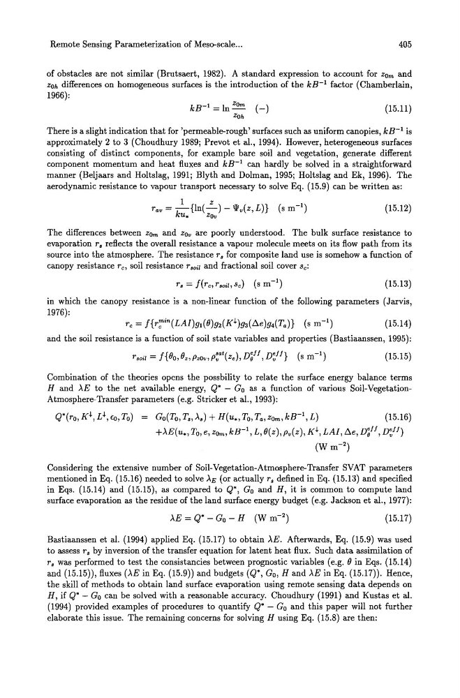
kB- l = In ZOrn ( _)
ZOh
(15.11)
There is a slight indication that for 'permeable-rough' surfaces such as uniform canopies, kB- l is
approximately 2 to 3 (Choudhury 1989; Prevot et al., 1994). However, heterogeneous surfaces
consisting of distinct components, for example bare soil and vegetation, generate different
component momentum and heat fluxes and kB- l can hardly be solved in a straightforward
manner (Beljaars and Holtslag, 1991; Blyth and Dolman, 1995; Holtslag and Ek, 1996). The
aerodynamic resistance to vapour transport necessary to solve Eq. (15.9) can be written as:
1
Z
rav=-k {In(-)-Wv(z,L)} (sm- l )
u.
ZOv
(15.12)
The differences between ZOrn and ZOv are poorly understood. The bulk surface resistance to
evaporation r. reflects the overall resistance a vapour molecule meets on its flow path from its
source into the atmosphere. The resistance r. for composite land use is somehow a function of
canopy resistance r e, soil resistance r .oil and fractional soil cover Se:
(15.13)
in which the canopy resistance is a non-linear function of the following parameters (Jarvis,
1976):
(15.14)
and the soil resistance is a function of soil state variables and properties (Bastiaanssen, 1995):
(15.15)
Combination of the theories opens the possbility to relate the surface energy balance terms
H and AE to the net available energy, Q* - Go as a function of various Soil-VegetationAtmosphere-Transfer parameters (e.g. Stricker et al., 1993):
(15.16)
+AE(u*, To, e, ZOrn, kB- l , L, B(z), Pv(z), K+, LA!, ~e, D~ff, D~JJ)
(W m- 2 )
Considering the extensive number of Soil-Vegetation-Atmosphere-Transfer SVAT parameters
mentioned in Eq. (15.16) needed to solve AE (or actually r. defined in Eq. (15.13) and specified
in Eqs. (15.14) and (15.15), as compared to Q*, Go and H, it is common to compute land
surface evaporation as the residue of the land surface energy budget (e.g. Jackson et aI., 1977):
(15.17)
Bastiaanssen et al. (1994) applied Eq. (15.17) to obtain AE. Afterwards, Eq. (15.9) was used
to assess rs by inversion of the transfer equation for latent heat flux. Such data assimilation of
rs was performed to test the consistancies between prognostic variables (e.g. Bin Eqs. (15.14)
and (15.15)), fluxes (AE in Eq. (15.9)) and budgets (Q*, Go, Hand AE in Eq. (15.17)). Hence,
the skill of methods to obtain land surface evaporation using remote sensing data depends on
H, if Q* - Go can be solved with a reasonable accuracy. Choudhury (1991) and Kustas et al.
(1994) provided examples of procedures to quantify Q* - Go and this paper will not further
elaborate this issue. The remaining concerns for solving H using Eq. (15.8) are then:
405
of obstacles are not similar (Brutsaert, 1982). A standard expression to account for ZOrn and
ZOh differences on homogeneous surfaces is the introduction of the kB- l factor (Chamberlain,
1966):
kB- l = In ZOrn ( _)
ZOh
(15.11)
There is a slight indication that for 'permeable-rough' surfaces such as uniform canopies, kB- l is
approximately 2 to 3 (Choudhury 1989; Prevot et al., 1994). However, heterogeneous surfaces
consisting of distinct components, for example bare soil and vegetation, generate different
component momentum and heat fluxes and kB- l can hardly be solved in a straightforward
manner (Beljaars and Holtslag, 1991; Blyth and Dolman, 1995; Holtslag and Ek, 1996). The
aerodynamic resistance to vapour transport necessary to solve Eq. (15.9) can be written as:
1
Z
rav=-k {In(-)-Wv(z,L)} (sm- l )
u.
ZOv
(15.12)
The differences between ZOrn and ZOv are poorly understood. The bulk surface resistance to
evaporation r. reflects the overall resistance a vapour molecule meets on its flow path from its
source into the atmosphere. The resistance r. for composite land use is somehow a function of
canopy resistance r e, soil resistance r .oil and fractional soil cover Se:
(15.13)
in which the canopy resistance is a non-linear function of the following parameters (Jarvis,
1976):
(15.14)
and the soil resistance is a function of soil state variables and properties (Bastiaanssen, 1995):
(15.15)
Combination of the theories opens the possbility to relate the surface energy balance terms
H and AE to the net available energy, Q* - Go as a function of various Soil-VegetationAtmosphere-Transfer parameters (e.g. Stricker et al., 1993):
(15.16)
+AE(u*, To, e, ZOrn, kB- l , L, B(z), Pv(z), K+, LA!, ~e, D~ff, D~JJ)
(W m- 2 )
Considering the extensive number of Soil-Vegetation-Atmosphere-Transfer SVAT parameters
mentioned in Eq. (15.16) needed to solve AE (or actually r. defined in Eq. (15.13) and specified
in Eqs. (15.14) and (15.15), as compared to Q*, Go and H, it is common to compute land
surface evaporation as the residue of the land surface energy budget (e.g. Jackson et aI., 1977):
(15.17)
Bastiaanssen et al. (1994) applied Eq. (15.17) to obtain AE. Afterwards, Eq. (15.9) was used
to assess rs by inversion of the transfer equation for latent heat flux. Such data assimilation of
rs was performed to test the consistancies between prognostic variables (e.g. Bin Eqs. (15.14)
and (15.15)), fluxes (AE in Eq. (15.9)) and budgets (Q*, Go, Hand AE in Eq. (15.17)). Hence,
the skill of methods to obtain land surface evaporation using remote sensing data depends on
H, if Q* - Go can be solved with a reasonable accuracy. Choudhury (1991) and Kustas et al.
(1994) provided examples of procedures to quantify Q* - Go and this paper will not further
elaborate this issue. The remaining concerns for solving H using Eq. (15.8) are then: