

382
S. Paloscia
1.00
@
Ii
8
0.90
co
...
:J
+'
IB
I '
0
GiO.80
a.
E
co
I-- 0.70
, ,.o.1B
.0.'
.0.
,
.0. , , ,
" IB
"0
co
N
"
IB
.0.
•
~0.60
IB
'0
z 0.50
0.40 0
10
20
30
SMC~
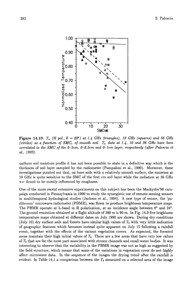
Figure 14.10: Tn (H pol., () = 2(J') at 1.4 GHz (triangles), 10 GHz (squares) and 36 GHz
(circles) as a function of SMCv of smooth soil. Tn data at 1.4, 10 and 36 GHz have been
correlated to the SMC of the O-Scm, 0-2.Scm and 0-lcm layer, respectively (after Paloscia et
al., 1993).
uniform soil moisture profile it has not been possible to state in a definitive way which is the
thickness of soil layer sampled by the radiometer (Pampaloni et al., 1990). Moreover, these
investigations pointed out that, on bare soils with a relatively smooth surface, the emission at
10 GHz is quite sensitive to the SMC of the first cm soil layer while the radiation at 36 GHz
wac found to be mostly influenced by roughness.
One of the more recent extensive experiments on this subject has been the Machydro'90 campaign conducted in Pennsylvania in 1990 to study the synergistic use of remote sensing sensors
in multitemporal hydrological studies (Jackson et al., 1994). A new type of sensor, the 'pushbroom' microwave radiometer (PBMR), was flown to produce brightness temperature maps.
The PBMR operate at L-band in H polarization, at an incidence angle between 8° and 24°.
The ground resolution obtained at a flight altitude of 300 m is 90 m. In Fig. 14.9 five brightness
temperature maps obtained at different dates on July 1990 are shown. During dry conditions
(July 10) dry surface soils and forests have similar high values of n with very little indication
of geographic features which becomes instead quite apparent on July 15 following a rainfall
event, together with the effects of the various vegetation covers. As expected, the forested
areas maintain their high initial values of n. There are a few areas that have very low values
of Tb that are for the most part associated with stream channels and small water bodies. It was
interesting to observe that the variability in the PBMR image was not as high as suggested by
the field structure, which means that some of the variations in vegetation cover do not highly
affect microwave data. In the sequence of the images the drying trend after the rainfall is
evident. In Table 14.1 a comparison between the n measured on a selected area of the image
S. Paloscia
1.00
@
Ii
8
0.90
co
...
:J
+'
IB
I '
0
GiO.80
a.
E
co
I-- 0.70
, ,.o.1B
.0.'
.0.
,
.0. , , ,
" IB
"0
co
N
"
IB
.0.
•
~0.60
IB
'0
z 0.50
0.40 0
10
20
30
SMC~
Figure 14.10: Tn (H pol., () = 2(J') at 1.4 GHz (triangles), 10 GHz (squares) and 36 GHz
(circles) as a function of SMCv of smooth soil. Tn data at 1.4, 10 and 36 GHz have been
correlated to the SMC of the O-Scm, 0-2.Scm and 0-lcm layer, respectively (after Paloscia et
al., 1993).
uniform soil moisture profile it has not been possible to state in a definitive way which is the
thickness of soil layer sampled by the radiometer (Pampaloni et al., 1990). Moreover, these
investigations pointed out that, on bare soils with a relatively smooth surface, the emission at
10 GHz is quite sensitive to the SMC of the first cm soil layer while the radiation at 36 GHz
wac found to be mostly influenced by roughness.
One of the more recent extensive experiments on this subject has been the Machydro'90 campaign conducted in Pennsylvania in 1990 to study the synergistic use of remote sensing sensors
in multitemporal hydrological studies (Jackson et al., 1994). A new type of sensor, the 'pushbroom' microwave radiometer (PBMR), was flown to produce brightness temperature maps.
The PBMR operate at L-band in H polarization, at an incidence angle between 8° and 24°.
The ground resolution obtained at a flight altitude of 300 m is 90 m. In Fig. 14.9 five brightness
temperature maps obtained at different dates on July 1990 are shown. During dry conditions
(July 10) dry surface soils and forests have similar high values of n with very little indication
of geographic features which becomes instead quite apparent on July 15 following a rainfall
event, together with the effects of the various vegetation covers. As expected, the forested
areas maintain their high initial values of n. There are a few areas that have very low values
of Tb that are for the most part associated with stream channels and small water bodies. It was
interesting to observe that the variability in the PBMR image was not as high as suggested by
the field structure, which means that some of the variations in vegetation cover do not highly
affect microwave data. In the sequence of the images the drying trend after the rainfall is
evident. In Table 14.1 a comparison between the n measured on a selected area of the image