

354
Eugene E. Clothiaux, Thomas P. Ackerman, David M. Babb
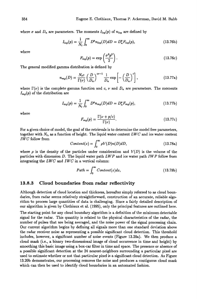
where a and Dn are parameters. The moments I/og(p) of n/og are defined by
(13.76b)
where
( a
2p2 )
F/og(p) = exp -2- .
(13.76c)
The general modified gamma distribution is defined by
Ntc (D )CV-l 1
[ ( D )C]
nmg(D) = rev) Dn
Dn exp - Dn
'
(13.77a)
where rev) is the complete gamma function and c, v and Dn are parameters. The moments
Img(P) of the distribution are
(13. 77b)
where
F. () _ r(v + pic)
mg p -
rev) .
(13.77c)
For a given choice of model, the goal of the retrievals is to determine the model free parameters,
together with Nt, as a function of height. The liquid water content LWC and ice water content
IW C follow from
Content(z) = 1
00 pV(D)n(D)dD,
(13.78a)
where p is the density of the particles under consideration and V(D) is the volume of the
particles with dimension D. The liquid water path LW P and ice water path IW P follow from
integrating the LWC and IWC in a vertical column:
Path = 1
00 Content(z)dz,
(13.78b)
13.8.3 Cloud boundaries from radar reflectivity
Although detection of cloud location and thickness, hereafter simply referred to as cloud boundaries, from radar seems relatively straightforward, construction of an accurate, reliable algorithm to process large quantities of data is challenging. Since a fairly detailed description of
our algorithm is given by Clothiaux et al. (1995), only the principal features are outlined here.
The starting point for any cloud boundary algorithm is a definition of the minimum detectable
signal for the radar. This quantity is related to the physical characteristics of the radar, the
number of pulses that are being averaged, and the noise power of the signal processing chain.
Our current algorithm begins by defining all signals more than one standard deviation above
the radar receiver noise as representing a possible significant cloud detection. This threshold
includes, however, a significant number of noise events (Figure 13.20a). We then produce a
cloud mask (i.e., a binary two-dimensional image of cloud occurrence in time and height) by
smoothing this basic image using a box-car filter in time and space. The presence or absence of
a possible significant detection at the 24 nearest-neighbors surrounding a particular pixel are
used to estimate whether or not that particular pixel is a significant cloud detection. As Figure
13.20b demonstrates, our processing removes the noise and produces a contiguous cloud mask
which can then be used to identify cloud boundaries in an automated fashion.
Eugene E. Clothiaux, Thomas P. Ackerman, David M. Babb
where a and Dn are parameters. The moments I/og(p) of n/og are defined by
(13.76b)
where
( a
2p2 )
F/og(p) = exp -2- .
(13.76c)
The general modified gamma distribution is defined by
Ntc (D )CV-l 1
[ ( D )C]
nmg(D) = rev) Dn
Dn exp - Dn
'
(13.77a)
where rev) is the complete gamma function and c, v and Dn are parameters. The moments
Img(P) of the distribution are
(13. 77b)
where
F. () _ r(v + pic)
mg p -
rev) .
(13.77c)
For a given choice of model, the goal of the retrievals is to determine the model free parameters,
together with Nt, as a function of height. The liquid water content LWC and ice water content
IW C follow from
Content(z) = 1
00 pV(D)n(D)dD,
(13.78a)
where p is the density of the particles under consideration and V(D) is the volume of the
particles with dimension D. The liquid water path LW P and ice water path IW P follow from
integrating the LWC and IWC in a vertical column:
Path = 1
00 Content(z)dz,
(13.78b)
13.8.3 Cloud boundaries from radar reflectivity
Although detection of cloud location and thickness, hereafter simply referred to as cloud boundaries, from radar seems relatively straightforward, construction of an accurate, reliable algorithm to process large quantities of data is challenging. Since a fairly detailed description of
our algorithm is given by Clothiaux et al. (1995), only the principal features are outlined here.
The starting point for any cloud boundary algorithm is a definition of the minimum detectable
signal for the radar. This quantity is related to the physical characteristics of the radar, the
number of pulses that are being averaged, and the noise power of the signal processing chain.
Our current algorithm begins by defining all signals more than one standard deviation above
the radar receiver noise as representing a possible significant cloud detection. This threshold
includes, however, a significant number of noise events (Figure 13.20a). We then produce a
cloud mask (i.e., a binary two-dimensional image of cloud occurrence in time and height) by
smoothing this basic image using a box-car filter in time and space. The presence or absence of
a possible significant detection at the 24 nearest-neighbors surrounding a particular pixel are
used to estimate whether or not that particular pixel is a significant cloud detection. As Figure
13.20b demonstrates, our processing removes the noise and produces a contiguous cloud mask
which can then be used to identify cloud boundaries in an automated fashion.