

342
Eugene E. Clothiaux, Thomas P. Ackerman, David M. Babb
only liquid water, we assume that the drops are liquid water spheres. Therefore, the theory
for scattering from spherical particles, i.e., Mie theory, is an appropriate tool to calculate the
scattering amplitude matrix element S2(180° ) of the drops as a function of size. The equations
for computing S2(180° ) come from Bohren and Huffman (1983); in fact, Bohren and Huffman
(BH, 4.6) provide the equation for S2(1800) and they also provide code that computes S2(1800)
(BH, Appendix A). Once the location r(i,i) and scattering matrix element S2(1800) are computed
for each particle, we compute the resulting voltage amplitude V(i,i) using (13.49b). We then
calculate the I and Q voltages using (13.52) with time t = O. To simulate the particles falling
within the resolution volume, we simply must advance the time t in (13.52). Since we must
take snapshots of the I and Q voltages at the pulse repitition frequency fprj of the radar, we
advance the time in increments of T. = il fprj. The Doppler shifts in (13.52) are related to the
particle fall velocities by
(13.54)
In the simulation we assume that the particle fall speeds are related to the particle drop diameter
by
_ {
4D(1 - e- 12D ),
v -
9.65 _ 1O.43e-o.6D,
if D < .75mm;
if .75mm < D,
(13.55)
where D is the diameter of the particle in mm and the velocity v has units of mls (Rogers et
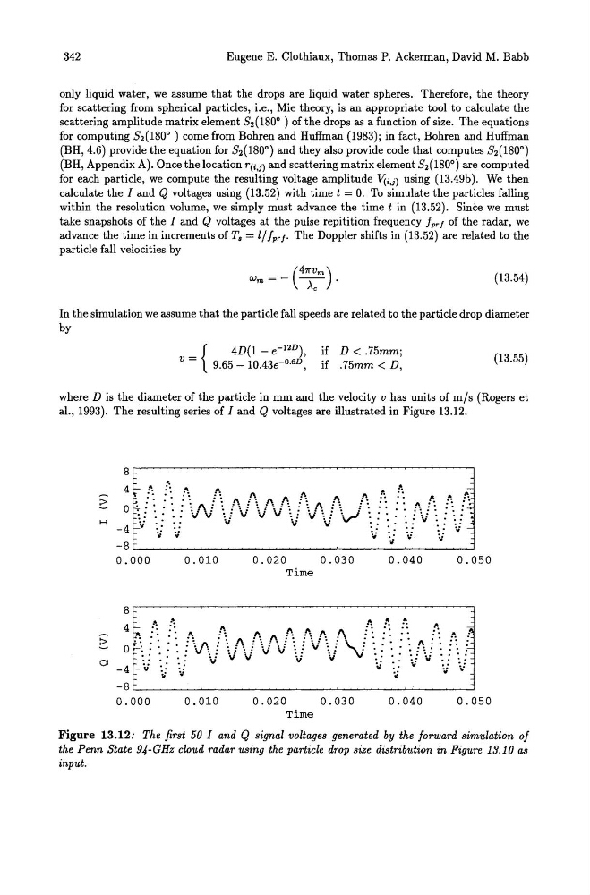
al., 1993). The resulting series of I and Q voltages are illustrated in Figure 13.12.
8
4:-: .... =:
:>
:". . r...
1\
!\
.!'. !-. ::
"," .
t \ : : A t .. ::
l\
!'.l':! . . . :~
o ~: : \/V J V V V \! \f\v! V \ . : : V . .
H
_4-v :;
•
'. :: v" -.;
;; ~ V -.;
-8~ ________ ~ ________ ~ ________ ~ ________________ ~
0.000
0.010
0.020
0.030
0.040
0.050
Time
8r-------~-----------------------------------.
: ~ t
".i v4?:
:~
2: o ;-:
QI -4 -v ;;
~
!:.
'.
-8
0.000
0.010
0.020
0.030
0.040
0.050
Time
Figure 13.12: The first 50 I and Q signal voltages generated by the forward simulation of
the Penn State 94-GHz cloud radar using the particle drop size distribution in Figure 13.10 as
input.
Eugene E. Clothiaux, Thomas P. Ackerman, David M. Babb
only liquid water, we assume that the drops are liquid water spheres. Therefore, the theory
for scattering from spherical particles, i.e., Mie theory, is an appropriate tool to calculate the
scattering amplitude matrix element S2(180° ) of the drops as a function of size. The equations
for computing S2(180° ) come from Bohren and Huffman (1983); in fact, Bohren and Huffman
(BH, 4.6) provide the equation for S2(1800) and they also provide code that computes S2(1800)
(BH, Appendix A). Once the location r(i,i) and scattering matrix element S2(1800) are computed
for each particle, we compute the resulting voltage amplitude V(i,i) using (13.49b). We then
calculate the I and Q voltages using (13.52) with time t = O. To simulate the particles falling
within the resolution volume, we simply must advance the time t in (13.52). Since we must
take snapshots of the I and Q voltages at the pulse repitition frequency fprj of the radar, we
advance the time in increments of T. = il fprj. The Doppler shifts in (13.52) are related to the
particle fall velocities by
(13.54)
In the simulation we assume that the particle fall speeds are related to the particle drop diameter
by
_ {
4D(1 - e- 12D ),
v -
9.65 _ 1O.43e-o.6D,
if D < .75mm;
if .75mm < D,
(13.55)
where D is the diameter of the particle in mm and the velocity v has units of mls (Rogers et
al., 1993). The resulting series of I and Q voltages are illustrated in Figure 13.12.
8
4:-: .... =:
:>
:". . r...
1\
!\
.!'. !-. ::
"," .
t \ : : A t .. ::
l\
!'.l':! . . . :~
o ~: : \/V J V V V \! \f\v! V \ . : : V . .
H
_4-v :;
•
'. :: v" -.;
;; ~ V -.;
-8~ ________ ~ ________ ~ ________ ~ ________________ ~
0.000
0.010
0.020
0.030
0.040
0.050
Time
8r-------~-----------------------------------.
: ~ t
".i v4?:
:~
2: o ;-:
QI -4 -v ;;
~
!:.
'.
-8
0.000
0.010
0.020
0.030
0.040
0.050
Time
Figure 13.12: The first 50 I and Q signal voltages generated by the forward simulation of
the Penn State 94-GHz cloud radar using the particle drop size distribution in Figure 13.10 as
input.