

332
Eugene E. Clothiaux, Thomas P. Ackerman, David M. Babb
where we have incorporated attenuation from the object to the radar receiver. The primes in
the definition of u indicate that the receiver antenna may not be collocated with the transmitter antenna. However, for most radar applications the transmitter and receiver antennas
are collocated. In this case, we are interested in only the backscatter cross section and we set
U(O/, A'(r, 0, PtGtTJOUb MO, 87r2ltlr
r
for the scattered field amplitude at the receiver antenna.
(13.17)
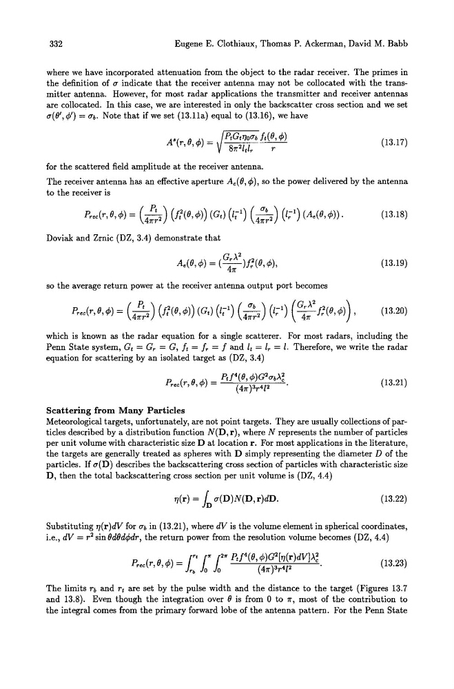
The receiver antenna has an effective aperture Ae( 0, to the receiver is
(13.18)
Doviak and Zrnic (DZ, 3.4) demonstrate that
(13.19)
so the average return power at the receiver antenna output port becomes
(13.20)
which is known as the radar equation for a single scatterer. For most radars, including the
Penn State system, Gt = Gr = G, It = Ir = I and It = lr = l. Therefore, we write the radar
equation for scattering by an isolated target as (DZ, 3.4)
(13.21 )
Scattering from Many Particles
Meteorological targets, unfortunately, are not point targets. They are usually collections of particles described by a distribution function N(D, r), where N represents the number of particles
per unit volume with characteristic size D at location r. For most applications in the literature,
the targets are generally treated as spheres with D simply representing the diameter D of the
particles. If u(D) describes the backscattering cross section of particles with characteristic size
D, then the total backscattering cross section per unit volume is (DZ, 4.4)
TJ(r) = in u(D)N(D,r)dD.
(13.22)
Substituting l7(r)dV for Ub in (13.21), where dV is the volume element in spherical coordinates,
i.e., dV = r2 sin OdOd (13.23)
The limits rb and rt are set by the pulse width and the distance to the target (Figures 13.7
and 13.8). Even though the integration over 0 is from 0 to 7r, most of the contribution to
the integral comes from the primary forward lobe of the antenna pattern. For the Penn State
Eugene E. Clothiaux, Thomas P. Ackerman, David M. Babb
where we have incorporated attenuation from the object to the radar receiver. The primes in
the definition of u indicate that the receiver antenna may not be collocated with the transmitter antenna. However, for most radar applications the transmitter and receiver antennas
are collocated. In this case, we are interested in only the backscatter cross section and we set
U(O/, A'(r, 0, PtGtTJOUb MO, 87r2ltlr
r
for the scattered field amplitude at the receiver antenna.
(13.17)
The receiver antenna has an effective aperture Ae( 0, to the receiver is
(13.18)
Doviak and Zrnic (DZ, 3.4) demonstrate that
(13.19)
so the average return power at the receiver antenna output port becomes
(13.20)
which is known as the radar equation for a single scatterer. For most radars, including the
Penn State system, Gt = Gr = G, It = Ir = I and It = lr = l. Therefore, we write the radar
equation for scattering by an isolated target as (DZ, 3.4)
(13.21 )
Scattering from Many Particles
Meteorological targets, unfortunately, are not point targets. They are usually collections of particles described by a distribution function N(D, r), where N represents the number of particles
per unit volume with characteristic size D at location r. For most applications in the literature,
the targets are generally treated as spheres with D simply representing the diameter D of the
particles. If u(D) describes the backscattering cross section of particles with characteristic size
D, then the total backscattering cross section per unit volume is (DZ, 4.4)
TJ(r) = in u(D)N(D,r)dD.
(13.22)
Substituting l7(r)dV for Ub in (13.21), where dV is the volume element in spherical coordinates,
i.e., dV = r2 sin OdOd (13.23)
The limits rb and rt are set by the pulse width and the distance to the target (Figures 13.7
and 13.8). Even though the integration over 0 is from 0 to 7r, most of the contribution to
the integral comes from the primary forward lobe of the antenna pattern. For the Penn State