

Lidar Measurements: Atmospheric Constituents ...
221
9.0
8.5
E
-'<
8.0
o--C
I
(?
W
7.5
I
7.0
6.5 a
0.25
0.5
0.75
1
a 0.025 0.05 0.075 0.1
a
6
12
18
24
EXTINCTION COEF. km- 1
BACKSC. COEF .. km- 1 sr- 1
LlDAR RATIO. sr
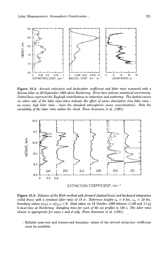
Figure 10.2: Aerosol extinction and backscatter coefficient and lidar ratio measured with a
Raman lidar on 20 September 1989 above Norderney. Error bars indicate statistical uncertainty.
Dotted lines represent the Rayleigh contributions to extinction and scattering. The dashed curves
on either side of the lidar ratio trace indicate the effect of ozone absorption (low lidar ratio -
no ozone, high lidar ratio - twice the standard atmospheric ozone concentration). Note the
variability of the lidar ratio within the cloud. From Ansmann et al. (1991).
12.5
11.7
E
.:::t.
10.9
f-..:'
:r: C)
W
10.1
:r:
9.3
(a)
(d)
(f)
8.5
0
0.4 0.8
EXTINCTION COEFFICIENT. km- 1
Figure 10.3: Solution of the Klett method with forward (dashed lines) and backward integration
(solid lines) with a constant lidar ratio of 13 sr. Reference heights Zo = 6 km, Zm = 12 km,
boundary values a(zo) = a(zm) = O. Data taken on 18 October 1989 between 11:29 and 11:44
h local time at Norderney. Sampling time for each of the six profiles is 150 s. The lidar ratio
chosen is appropriate for cases c and d only. From Ansmann et al. {1991}.
- Reliable near-end and remote-end boundary values of the aerosol extinction coefficient
must be available.
221
9.0
8.5
E
-'<
8.0
o--C
I
(?
W
7.5
I
7.0
6.5 a
0.25
0.5
0.75
1
a 0.025 0.05 0.075 0.1
a
6
12
18
24
EXTINCTION COEF. km- 1
BACKSC. COEF .. km- 1 sr- 1
LlDAR RATIO. sr
Figure 10.2: Aerosol extinction and backscatter coefficient and lidar ratio measured with a
Raman lidar on 20 September 1989 above Norderney. Error bars indicate statistical uncertainty.
Dotted lines represent the Rayleigh contributions to extinction and scattering. The dashed curves
on either side of the lidar ratio trace indicate the effect of ozone absorption (low lidar ratio -
no ozone, high lidar ratio - twice the standard atmospheric ozone concentration). Note the
variability of the lidar ratio within the cloud. From Ansmann et al. (1991).
12.5
11.7
E
.:::t.
10.9
f-..:'
:r: C)
W
10.1
:r:
9.3
(a)
(d)
(f)
8.5
0
0.4 0.8
EXTINCTION COEFFICIENT. km- 1
Figure 10.3: Solution of the Klett method with forward (dashed lines) and backward integration
(solid lines) with a constant lidar ratio of 13 sr. Reference heights Zo = 6 km, Zm = 12 km,
boundary values a(zo) = a(zm) = O. Data taken on 18 October 1989 between 11:29 and 11:44
h local time at Norderney. Sampling time for each of the six profiles is 150 s. The lidar ratio
chosen is appropriate for cases c and d only. From Ansmann et al. {1991}.
- Reliable near-end and remote-end boundary values of the aerosol extinction coefficient
must be available.