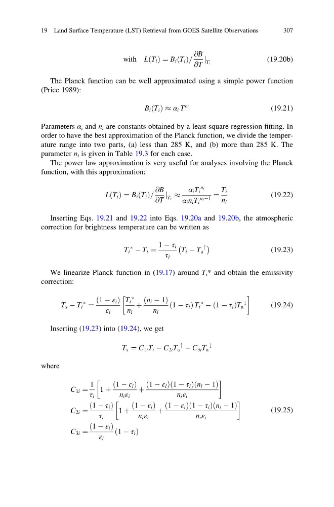
with L T i
ð Þ ¼ B i T i
ð Þ=
@B
@T
j T i
(19.20b)
The Planck function can be well approximated using a simple power function
(Price 1989):
B i T i
ð Þ % α i T
n i
(19.21)
Parameters α i and n i are constants obtained by a least-square regression fitting. In
order to have the best approximation of the Planck function, we divide the temperature range into two parts, (a) less than 285 K, and (b) more than 285 K. The
parameter n i is given in Table 19.3 for each case.
The power law approximation is very useful for analyses involving the Planck
function, with this approximation:
L T i
ð Þ ¼ B i T i
ð Þ=
@B
@T
j T i %
α i T i
n i
α i n i T i
n i À1
¼
T i
n i
(19.22)
Inserting Eqs. 19.21 and 19.22 into Eqs. 19.20a and 19.20b, the atmospheric
correction for brightness temperature can be written as
T i
Ã
À T i ¼
1 À τ i
τ i
T i À T a
"
À
Á
(19.23)
We linearize Planck function in (19.17) around T i * and obtain the emissivity
correction:
T s À T i
Ã
¼
1 À ε i
ð
Þ
ε i
T i
Ã
n i
þ
n i À 1
ð
Þ
n i
1 À τ i
ð
ÞT i
Ã
À 1 À τ i
ð
ÞT a
#
!
(19.24)
Inserting (19.23) into (19.24), we get
T s ¼ C 1i T i À C 2i T a
"
À C 3i T a
#
where
C 1i ¼
1
τ i
1 þ
1 À ε i
ð
Þ
n i ε i
þ
1 À ε i
ð
Þ 1 À τ i
ð
Þ n i À 1
ð
Þ
n i ε i
!
C 2i ¼
1 À τ i
ð
Þ
τ i
1 þ
1 À ε i
ð
Þ
n i ε i
þ
1 À ε i
ð
Þ 1 À τ i
ð
Þ n i À 1
ð
Þ
n i ε i
!
C 3i ¼
1 À ε i
ð
Þ
ε i
1 À τ i
ð
Þ
(19.25)
19 Land Surface Temperature (LST) Retrieval from GOES Satellite Observations
307