

difference time series of the gridded temperature. In this approach, a series of sensitivity experiments were conducted in which μ N10 changed in a reasonable range [e.g.,
0–12.5 (sr m
2 cm
À1
) (mW)
À1 for all MSU channels]. For each given μ N10 , a set of
calibration coefficients for all other satellites were obtained sequentially from
regressions of their SNO matchups. These calibration coefficients were then applied
globally to every observation footprint to obtain a Level-1c radiance dataset for each
satellite from Eq. (8.1). Next, a limb correction was applied to adjust different incident
angles of the off-nadir footprints to the nadir direction, and global ocean-mean
brightness temperatures were further obtained by averaging seven near-nadir, limbcorrected radiances for each sensitivity experiment. Similar to Fig. 8.3, the ocean-mean
data are used here for evaluating inter-satellite radiance biases that are related to
instrument temperature variability.
The global ocean-mean inter-satellite bias variability, as measured by the mean
standard deviation (σ m ) of the inter-satellite difference time series for all satellite
pairs, is evaluated for all the sensitivity experiments. Figure 8.5 shows σ m versus
μ N10 for all the sensitivity experiments. The quantity σ is a measurement of
instrument calibration errors related to the instrument temperature signals in the
radiance datasets. Figure 8.3 showed an example of this quantity for a particular
satellite pair. The final calibration point for μ N10 is selected when the mean
instrument calibration error is minimized.
The new calibration coefficients resulted in a FCDR with much smaller solar
heating-related calibration errors compared to the prelaunch calibration. Figure 8.6
shows a similar global ocean-mean inter-satellite brightness temperature difference
time series as in Fig. 8.3 except for the SNO-calibrated radiances. As seen, the
instrument temperature-related variability as observed in Fig. 8.3 for NOAA-10
through NOAA-14 is mostly removed, and their inter-satellite biases are significantly reduced. Quantitatively, the inter-satellite biases and σ m for the SNO
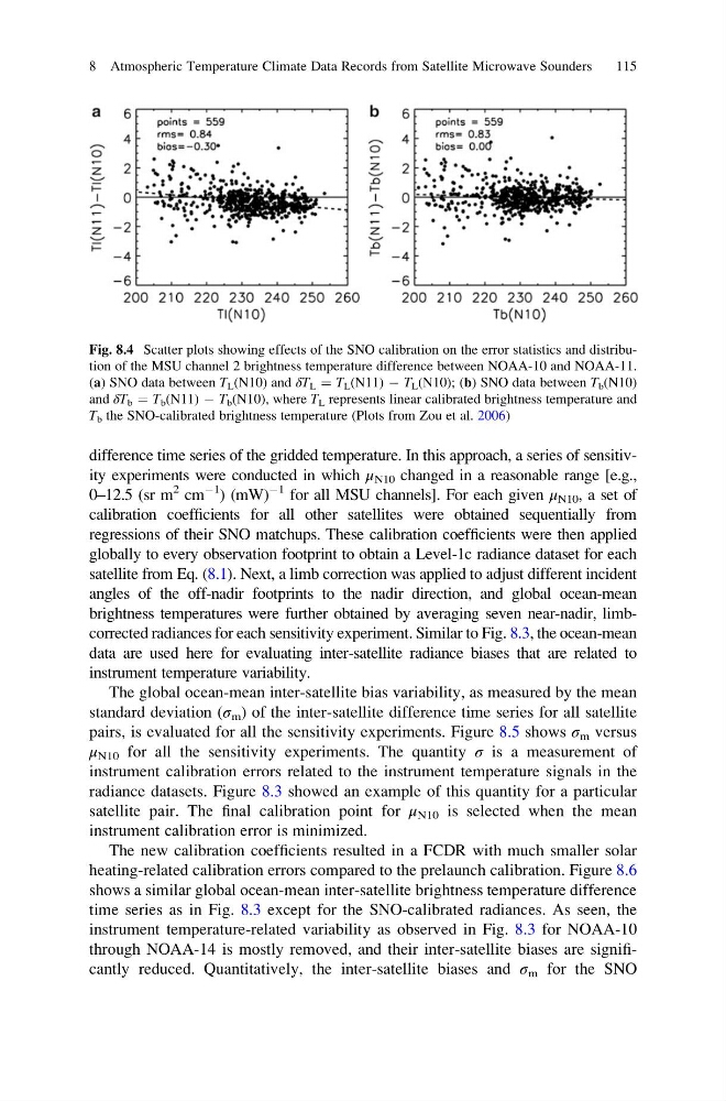
Fig. 8.4 Scatter plots showing effects of the SNO calibration on the error statistics and distribution of the MSU channel 2 brightness temperature difference between NOAA-10 and NOAA-11.
(a) SNO data between T L (N10) and δT L ¼ T L (N11) À T L (N10); (b) SNO data between T b (N10)
and δT b ¼ T b (N11) À T b (N10), where T L represents linear calibrated brightness temperature and
T b the SNO-calibrated brightness temperature (Plots from Zou et al. 2006)
8 Atmospheric Temperature Climate Data Records from Satellite Microwave Sounders
115
0–12.5 (sr m
2 cm
À1
) (mW)
À1 for all MSU channels]. For each given μ N10 , a set of
calibration coefficients for all other satellites were obtained sequentially from
regressions of their SNO matchups. These calibration coefficients were then applied
globally to every observation footprint to obtain a Level-1c radiance dataset for each
satellite from Eq. (8.1). Next, a limb correction was applied to adjust different incident
angles of the off-nadir footprints to the nadir direction, and global ocean-mean
brightness temperatures were further obtained by averaging seven near-nadir, limbcorrected radiances for each sensitivity experiment. Similar to Fig. 8.3, the ocean-mean
data are used here for evaluating inter-satellite radiance biases that are related to
instrument temperature variability.
The global ocean-mean inter-satellite bias variability, as measured by the mean
standard deviation (σ m ) of the inter-satellite difference time series for all satellite
pairs, is evaluated for all the sensitivity experiments. Figure 8.5 shows σ m versus
μ N10 for all the sensitivity experiments. The quantity σ is a measurement of
instrument calibration errors related to the instrument temperature signals in the
radiance datasets. Figure 8.3 showed an example of this quantity for a particular
satellite pair. The final calibration point for μ N10 is selected when the mean
instrument calibration error is minimized.
The new calibration coefficients resulted in a FCDR with much smaller solar
heating-related calibration errors compared to the prelaunch calibration. Figure 8.6
shows a similar global ocean-mean inter-satellite brightness temperature difference
time series as in Fig. 8.3 except for the SNO-calibrated radiances. As seen, the
instrument temperature-related variability as observed in Fig. 8.3 for NOAA-10
through NOAA-14 is mostly removed, and their inter-satellite biases are significantly reduced. Quantitatively, the inter-satellite biases and σ m for the SNO
Fig. 8.4 Scatter plots showing effects of the SNO calibration on the error statistics and distribution of the MSU channel 2 brightness temperature difference between NOAA-10 and NOAA-11.
(a) SNO data between T L (N10) and δT L ¼ T L (N11) À T L (N10); (b) SNO data between T b (N10)
and δT b ¼ T b (N11) À T b (N10), where T L represents linear calibrated brightness temperature and
T b the SNO-calibrated brightness temperature (Plots from Zou et al. 2006)
8 Atmospheric Temperature Climate Data Records from Satellite Microwave Sounders
115