

Spatial and Temporal Variations in Precipitation and Aridity Index Series of Turkey
187
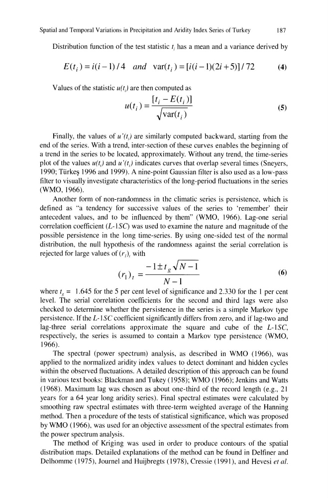
Distribution function of the test statistic ti has a mean and a variance derived by
E(t i ) = i(i -1) /4 and var(t i ) = [i(i -1)(2i + 5)] / 72
(4)
Values of the statistic u(t) are then computed as
[t i - E(t i )]
u(t.) =
(5)
I
~var(ti)
Finally, the values of u '(t) are similarly computed backward, starting from the
end of the series. With a trend, inter-section of these curves enables the beginning of
a trend in the series to be located, approximately. Without any trend, the time-series
plot of the values u(t) and u'(t) indicates curves that overlap several times (Sneyers,
1990; Ti.irke~ 1996 and 1999). A nine-point Gaussian filter is also used as a low-pass
filter to visually investigate characteristics of the long-period tluctuations in the series
(WMO, 1966).
Another form of non-randomness in the climatic series is persistence, which is
defined as "a tendency for successive values of the series to 'remember' their
antecedent values, and to be intluenced by them" (WMO, 1966). Lag-one serial
correlation coefficient (L-l SC) was used to examine the nature and magnitude of the
possible persistence in the long time-series. By using one-sided test of the normal
distribution, the null hypothesis of the randomness against the serial correlation is
rejected for large values of (r,), with
-l±tg-JN-I
(r] ) t =
(6)
N-I
where tg = 1.645 for the 5 per cent level of significance and 2.330 for the I per cent
level. The serial correlation coefficients for the second and third lags were also
checked to determine whether the persistence in the series is a simple Markov type
persistence. If the L-I SC coefficient significantly differs from zero, and if lag-two and
lag-three serial correlations approximate the square and cube of the L-ISC,
respectively, the series is assumed to contain a Markov type persistence (WMO,
1966).
The spectral (power spectrum) analysis, as described in WMO (1966), was
applied to the normalized aridity index values to detect dominant and hidden cycles
within the observed tluctuations. A detailed description of this approach can be found
in various text books: Blackman and Tukey (1958); WMO (1966); Jenkins and Watts
(1968). Maximum lag was chosen as about one-third of the record length (e.g., 21
years for a 64 year long aridity series). Final spectral estimates were calculated by
smoothing raw spectral estimates with three-term weighted average of the Hanning
method. Then a procedure of the tests of statistical significance, which was proposed
by WMO (1966), was used for an objective assessment of the spectral estimates from
the power spectrum analysis.
The method of Kriging was used in order to produce contours of the spatial
distribution maps. Detailed explanations of the method can be found in Delfiner and
Delhomme (1975), Journel and Huijbregts (1978), Cressie (1991), and Hevesi et al.
187
Distribution function of the test statistic ti has a mean and a variance derived by
E(t i ) = i(i -1) /4 and var(t i ) = [i(i -1)(2i + 5)] / 72
(4)
Values of the statistic u(t) are then computed as
[t i - E(t i )]
u(t.) =
(5)
I
~var(ti)
Finally, the values of u '(t) are similarly computed backward, starting from the
end of the series. With a trend, inter-section of these curves enables the beginning of
a trend in the series to be located, approximately. Without any trend, the time-series
plot of the values u(t) and u'(t) indicates curves that overlap several times (Sneyers,
1990; Ti.irke~ 1996 and 1999). A nine-point Gaussian filter is also used as a low-pass
filter to visually investigate characteristics of the long-period tluctuations in the series
(WMO, 1966).
Another form of non-randomness in the climatic series is persistence, which is
defined as "a tendency for successive values of the series to 'remember' their
antecedent values, and to be intluenced by them" (WMO, 1966). Lag-one serial
correlation coefficient (L-l SC) was used to examine the nature and magnitude of the
possible persistence in the long time-series. By using one-sided test of the normal
distribution, the null hypothesis of the randomness against the serial correlation is
rejected for large values of (r,), with
-l±tg-JN-I
(r] ) t =
(6)
N-I
where tg = 1.645 for the 5 per cent level of significance and 2.330 for the I per cent
level. The serial correlation coefficients for the second and third lags were also
checked to determine whether the persistence in the series is a simple Markov type
persistence. If the L-I SC coefficient significantly differs from zero, and if lag-two and
lag-three serial correlations approximate the square and cube of the L-ISC,
respectively, the series is assumed to contain a Markov type persistence (WMO,
1966).
The spectral (power spectrum) analysis, as described in WMO (1966), was
applied to the normalized aridity index values to detect dominant and hidden cycles
within the observed tluctuations. A detailed description of this approach can be found
in various text books: Blackman and Tukey (1958); WMO (1966); Jenkins and Watts
(1968). Maximum lag was chosen as about one-third of the record length (e.g., 21
years for a 64 year long aridity series). Final spectral estimates were calculated by
smoothing raw spectral estimates with three-term weighted average of the Hanning
method. Then a procedure of the tests of statistical significance, which was proposed
by WMO (1966), was used for an objective assessment of the spectral estimates from
the power spectrum analysis.
The method of Kriging was used in order to produce contours of the spatial
distribution maps. Detailed explanations of the method can be found in Delfiner and
Delhomme (1975), Journel and Huijbregts (1978), Cressie (1991), and Hevesi et al.