

90
where L * is the adjoint of L with respect to the energy inner product. Note
that if L is represented in matrix form, then L * is just the matrix transpose
ofL.
Unlike L itself, the operator L*L (sometimes referred to as the Oseledec
operator, e.g. Abarbanel et al., 1991) is easily shown to be symmetric.
Hence its eigenvectors Vi(tO) can be chosen to form an orthonormal basis
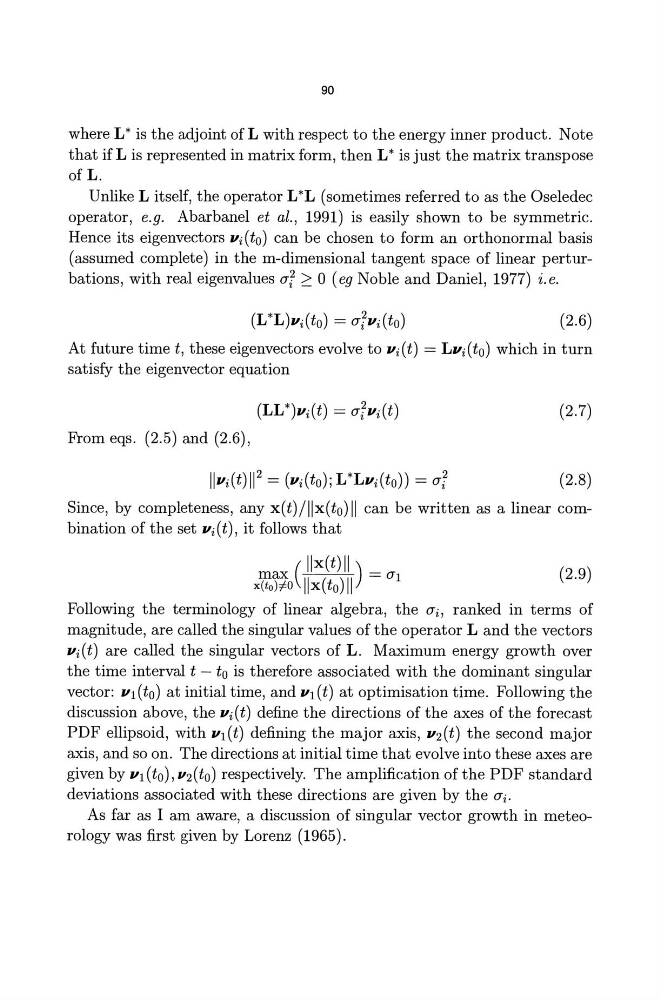
(assumed complete) in the m-dimensional tangent space of linear perturbations, with real eigenvalues 0"7 ~ 0 (eg Noble and Daniel, 1977) i. e.
(2.6)
At future time t, these eigenvectors evolve to Vi(t) = LVi(tO) which in turn
satisfy the eigenvector equation
(LL*)Vi(t) = O";Vi(t)
From eqs. (2.5) and (2.6),
(2.7)
(2.8)
Since, by completeness, any x(t)/llx(to)11 can be written as a linear combination of the set Vi (t), it follows that
max ( Ilx( t) II ) = O"I
x(to):fo Ilx(to) II
(2.9)
Following the terminology of linear algebra, the O"i, ranked in terms of
magnitude, are called the singular values of the operator L and the vectors
Vi(t) are called the singular vectors of L. Maximum energy growth over
the time interval t - to is therefore associated with the dominant singular
vector: VI (to) at initial time, and VI (t) at optimisation time. Following the
discussion above, the Vi(t) define the directions of the axes of the forecast
PDF ellipsoid, with VI(t) defining the major axis, V2(t) the second major
axis, and so on. The directions at initial time that evolve into these axes are
given by VI(tO),V2(tO) respectively. The amplification ofthe PDF standard
deviations associated with these directions are given by the O"i.
As far as I am aware, a discussion of singular vector growth in meteorology was first given by Lorenz (1965).
where L * is the adjoint of L with respect to the energy inner product. Note
that if L is represented in matrix form, then L * is just the matrix transpose
ofL.
Unlike L itself, the operator L*L (sometimes referred to as the Oseledec
operator, e.g. Abarbanel et al., 1991) is easily shown to be symmetric.
Hence its eigenvectors Vi(tO) can be chosen to form an orthonormal basis
(assumed complete) in the m-dimensional tangent space of linear perturbations, with real eigenvalues 0"7 ~ 0 (eg Noble and Daniel, 1977) i. e.
(2.6)
At future time t, these eigenvectors evolve to Vi(t) = LVi(tO) which in turn
satisfy the eigenvector equation
(LL*)Vi(t) = O";Vi(t)
From eqs. (2.5) and (2.6),
(2.7)
(2.8)
Since, by completeness, any x(t)/llx(to)11 can be written as a linear combination of the set Vi (t), it follows that
max ( Ilx( t) II ) = O"I
x(to):fo Ilx(to) II
(2.9)
Following the terminology of linear algebra, the O"i, ranked in terms of
magnitude, are called the singular values of the operator L and the vectors
Vi(t) are called the singular vectors of L. Maximum energy growth over
the time interval t - to is therefore associated with the dominant singular
vector: VI (to) at initial time, and VI (t) at optimisation time. Following the
discussion above, the Vi(t) define the directions of the axes of the forecast
PDF ellipsoid, with VI(t) defining the major axis, V2(t) the second major
axis, and so on. The directions at initial time that evolve into these axes are
given by VI(tO),V2(tO) respectively. The amplification ofthe PDF standard
deviations associated with these directions are given by the O"i.
As far as I am aware, a discussion of singular vector growth in meteorology was first given by Lorenz (1965).