347
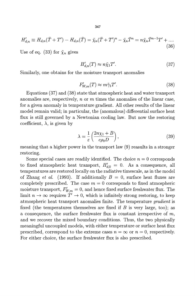
H~,n:= Hd,n(,T + T') - Hd,n("T) = Xn(T + T't - XnTn = nXntn-1T' + ....
(36)
Use of eq. (33) for Xn gives
(37)
Similarly, one obtains for the moisture transport anomalies
(38)
Equations (37) and (38) state that atmospheric heat and water transport
anomalies are, respectively, n or m times the anomalies of the linear case,
for a given anomaly in temperature gradient. All other results of the linear
model remain valid; in particular, the (anomalous) differential surface heat
flux is still governed by a Newtonian cooling law. But now the restoring
coefficient, .x, is given by
.x = ~ (2nXl + B) ,
c
cpoD
(39)
meaning that a higher power in the transport law (9) reasults in a stronger
restoring.
Some special cases are readily identified. The choice n = ° corresponds
to fixed atmospheric heat transport, Hd,o = 0. As a consequence, all
temperatures are restored locally on the radiative timescale, as in the model
of Zhang et al. (1993). If additionally B = 0, surface heat fluxes are
completely prescribed. The case m = ° corresponds to fixed atmospheric
moisture transport, F£Vm = 0, and hence fixed surface freshwater flux. The
limit n -+ 00 requires rT' -+ 0, which is infinitely strong restoring, to keep
atmospheric heat transport anomalies finite. The temperature gradient is
fixed (the temperatures themselves are fixed if B is very large, too); as
a consequence, the surface freshwater flux is constant irrespective of m,
and we recover the mixed boundary conditions. Thus, the two physically
meaningful uncoupled models, with either temperature or surface heat flux
prescribed, correspond to the extreme cases n = 00 or n = 0, respectively.
For either choice, the surface freshwater flux is also prescribed.