

170
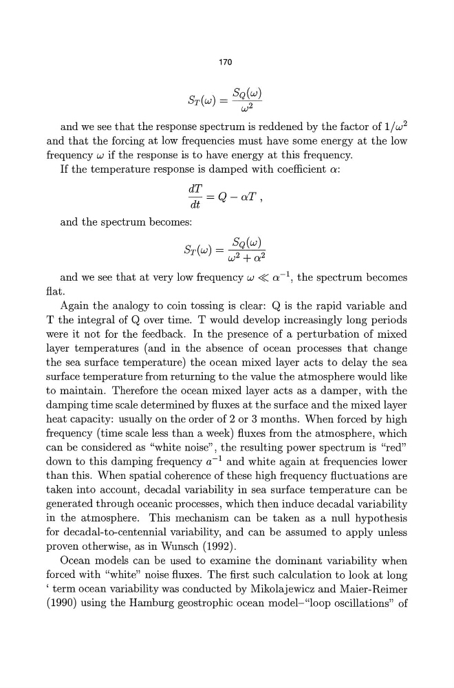
ST(W) = SQ(W)
w 2
and we see that the response spectrum is reddened by the factor of 1/w 2
and that the forcing at low frequencies must have some energy at the low
frequency W if the response is to have energy at this frequency.
If the temperature response is damped with coefficient a:
dT
di=Q-aT,
and the spectrum becomes:
ST(W) = Sdw)
w 2 +a 2
and we see that at very low frequency w « a-I, the spectrum becomes
flat.
Again the analogy to coin tossing is clear: Q is the rapid variable and
T the integral of Q over time. T would develop increasingly long periods
were it not for the feedback. In the presence of a perturbation of mixed
layer temperatures (and in the absence of ocean processes that change
the sea surface temperature) the ocean mixed layer acts to delay the sea
surface temperature from returning to the value the atmosphere would like
to maintain. Therefore the ocean mixed layer acts as a damper, with the
damping time scale determined by fluxes at the surface and the mixed layer
heat capacity: usually on the order of 2 or 3 months. When forced by high
frequency (time scale less than a week) fluxes from the atmosphere, which
can be considered as "white noise" , the resulting power spectrum is "red"
down to this damping frequency a-I and white again at frequencies lower
than this. When spatial coherence of these high frequency fluctuations are
taken into account, decadal variability in sea surface temperature can be
generated through oceanic processes, which then induce decadal variability
in the atmosphere. This mechanism can be taken as a null hypothesis
for decadal-to-centennial variability, and can be assumed to apply unless
proven otherwise, as in Wunsch (1992).
Ocean models can be used to examine the dominant variability when
forced with "white" noise fluxes. The first such calculation to look at long
, term ocean variability was conducted by Mikolajewicz and Maier-Reimer
(1990) using the Hamburg geostrophic ocean model-"loop oscillations" of
ST(W) = SQ(W)
w 2
and we see that the response spectrum is reddened by the factor of 1/w 2
and that the forcing at low frequencies must have some energy at the low
frequency W if the response is to have energy at this frequency.
If the temperature response is damped with coefficient a:
dT
di=Q-aT,
and the spectrum becomes:
ST(W) = Sdw)
w 2 +a 2
and we see that at very low frequency w « a-I, the spectrum becomes
flat.
Again the analogy to coin tossing is clear: Q is the rapid variable and
T the integral of Q over time. T would develop increasingly long periods
were it not for the feedback. In the presence of a perturbation of mixed
layer temperatures (and in the absence of ocean processes that change
the sea surface temperature) the ocean mixed layer acts to delay the sea
surface temperature from returning to the value the atmosphere would like
to maintain. Therefore the ocean mixed layer acts as a damper, with the
damping time scale determined by fluxes at the surface and the mixed layer
heat capacity: usually on the order of 2 or 3 months. When forced by high
frequency (time scale less than a week) fluxes from the atmosphere, which
can be considered as "white noise" , the resulting power spectrum is "red"
down to this damping frequency a-I and white again at frequencies lower
than this. When spatial coherence of these high frequency fluctuations are
taken into account, decadal variability in sea surface temperature can be
generated through oceanic processes, which then induce decadal variability
in the atmosphere. This mechanism can be taken as a null hypothesis
for decadal-to-centennial variability, and can be assumed to apply unless
proven otherwise, as in Wunsch (1992).
Ocean models can be used to examine the dominant variability when
forced with "white" noise fluxes. The first such calculation to look at long
, term ocean variability was conducted by Mikolajewicz and Maier-Reimer
(1990) using the Hamburg geostrophic ocean model-"loop oscillations" of