

140
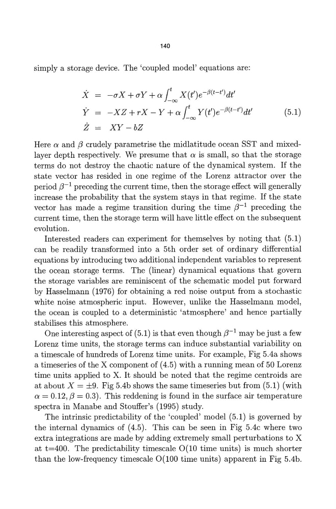
simply a storage device. The 'coupled model' equations are:
x
Y
Z
-CTX + CTY + a foo X(t')e-(3(t-t')dt'
-XZ + r X - Y + a foo Y(t') e-(3(t-t') dt'
XY-bZ
(5.1)
Here a and j3 crudely parametrise the midlatitude ocean SST and mixedlayer depth respectively. We presume that a is small, so that the storage
terms do not destroy the chaotic nature of the dynamical system. If the
state vector has resided in one regime of the Lorenz attractor over the
period j3-1 preceding the current time, then the storage effect will generally
increase the probability that the system stays in that regime. If the state
vector has made a regime transition during the time j3-1 preceding the
current time, then the storage term will have little effect on the subsequent
evolution.
Interested readers can experiment for themselves by noting that (5.1)
can be readily transformed into a 5th order set of ordinary differential
equations by introducing two additional independent variables to represent
the ocean storage terms. The (linear) dynamical equations that govern
the storage variables are reminiscent of the schematic model put forward
by Hasselmann (1976) for obtaining a red noise output from a stochastic
white noise atmospheric input. However, unlike the Hasselmann model,
the ocean is coupled to a deterministic 'atmosphere' and hence partially
stabilises this atmosphere.
One interesting aspect of (5.1) is that even though j3-1 may be just a few
Lorenz time units, the storage terms can induce substantial variability on
a timescale of hundreds of Lorenz time units. For example, Fig 5.4a shows
a timeseries of the X component of (4.5) with a running mean of 50 Lorenz
time units applied to X. It should be noted that the regime centroids are
at about X = ±9. Fig 5.4b shows the same timeseries but from (5.1) (with
a = 0.12, j3 = 0.3). This reddening is found in the surface air temperature
spectra in Manabe and Stouffer's (1995) study.
The intrinsic predictability of the 'coupled' model (5.1) is governed by
the internal dynamics of (4.5). This can be seen in Fig 5.4c where two
extra integrations are made by adding extremely small perturbations to X
at t=400. The predictability timescale 0(10 time units) is much shorter
than the low-frequency timescale 0(100 time units) apparent in Fig 5.4h.
simply a storage device. The 'coupled model' equations are:
x
Y
Z
-CTX + CTY + a foo X(t')e-(3(t-t')dt'
-XZ + r X - Y + a foo Y(t') e-(3(t-t') dt'
XY-bZ
(5.1)
Here a and j3 crudely parametrise the midlatitude ocean SST and mixedlayer depth respectively. We presume that a is small, so that the storage
terms do not destroy the chaotic nature of the dynamical system. If the
state vector has resided in one regime of the Lorenz attractor over the
period j3-1 preceding the current time, then the storage effect will generally
increase the probability that the system stays in that regime. If the state
vector has made a regime transition during the time j3-1 preceding the
current time, then the storage term will have little effect on the subsequent
evolution.
Interested readers can experiment for themselves by noting that (5.1)
can be readily transformed into a 5th order set of ordinary differential
equations by introducing two additional independent variables to represent
the ocean storage terms. The (linear) dynamical equations that govern
the storage variables are reminiscent of the schematic model put forward
by Hasselmann (1976) for obtaining a red noise output from a stochastic
white noise atmospheric input. However, unlike the Hasselmann model,
the ocean is coupled to a deterministic 'atmosphere' and hence partially
stabilises this atmosphere.
One interesting aspect of (5.1) is that even though j3-1 may be just a few
Lorenz time units, the storage terms can induce substantial variability on
a timescale of hundreds of Lorenz time units. For example, Fig 5.4a shows
a timeseries of the X component of (4.5) with a running mean of 50 Lorenz
time units applied to X. It should be noted that the regime centroids are
at about X = ±9. Fig 5.4b shows the same timeseries but from (5.1) (with
a = 0.12, j3 = 0.3). This reddening is found in the surface air temperature
spectra in Manabe and Stouffer's (1995) study.
The intrinsic predictability of the 'coupled' model (5.1) is governed by
the internal dynamics of (4.5). This can be seen in Fig 5.4c where two
extra integrations are made by adding extremely small perturbations to X
at t=400. The predictability timescale 0(10 time units) is much shorter
than the low-frequency timescale 0(100 time units) apparent in Fig 5.4h.