

137
Anomaly of yearly averaged THe Index
a) 2
1.6
..................... , ......... } ........ \ ... .
0.5
ili 0
-0.5
·1
.
. .
. " . .
·1.6 ........ : .......... , .......... ; .......... · .... · .... :· .... · .... ~ .... · .. · .. ;··· .. ·····1···· .. · .. T . . . . · . .
~
~
~
~
~
~
~
~
~
~
~
b) 1.5
cii .a.5
·1
·1.5
495
500
505
Ensemble II
510
515
520
525
530
Year
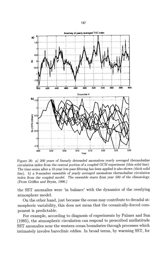
Figure 26: a) 200 years of linearly detrended anomalous yearly averaged thermohaline
circulation index from the central portion of a coupled GeM experiment (thin solid line).
The time series after a 10-year low-pass filtering has been applied is also shown (thick solid
line). b) a 9-member ensemble of yearly averaged anomalous thermohaline circulation
index from the coupled model. The ensemble starts from year 500 of the climatology.
(From Grimes and Bryan, 1996.)
the SST anomalies were 'in balance' with the dynamics of the overlying
atmosphere model.
On the other hand, just because the ocean may contribute to decadal atmospheric variability, this does not mean that the oceanically-forced component is predictable.
For example, according to diagnosis of experiments by Palmer and Sun
(1985), the atmospheric circulation can respond to prescribed midlatitude
SST anomalies near the western ocean boundaries through processes which
intimately involve baroclinic eddies. In broad terms, by warming SST, for
Anomaly of yearly averaged THe Index
a) 2
1.6
..................... , ......... } ........ \ ... .
0.5
ili 0
-0.5
·1
.
. .
. " . .
·1.6 ........ : .......... , .......... ; .......... · .... · .... :· .... · .... ~ .... · .. · .. ;··· .. ·····1···· .. · .. T . . . . · . .
~
~
~
~
~
~
~
~
~
~
~
b) 1.5
cii .a.5
·1
·1.5
495
500
505
Ensemble II
510
515
520
525
530
Year
Figure 26: a) 200 years of linearly detrended anomalous yearly averaged thermohaline
circulation index from the central portion of a coupled GeM experiment (thin solid line).
The time series after a 10-year low-pass filtering has been applied is also shown (thick solid
line). b) a 9-member ensemble of yearly averaged anomalous thermohaline circulation
index from the coupled model. The ensemble starts from year 500 of the climatology.
(From Grimes and Bryan, 1996.)
the SST anomalies were 'in balance' with the dynamics of the overlying
atmosphere model.
On the other hand, just because the ocean may contribute to decadal atmospheric variability, this does not mean that the oceanically-forced component is predictable.
For example, according to diagnosis of experiments by Palmer and Sun
(1985), the atmospheric circulation can respond to prescribed midlatitude
SST anomalies near the western ocean boundaries through processes which
intimately involve baroclinic eddies. In broad terms, by warming SST, for