

100
10,--------------------------------------------------,
,
9 ,
, , , , , , , , ,
"
o~--~----~--~----~--~~--~--~~--~----~--~
o
20
40
60
80
100
120
140
160
180
200
SingularlBreeding Vector Index
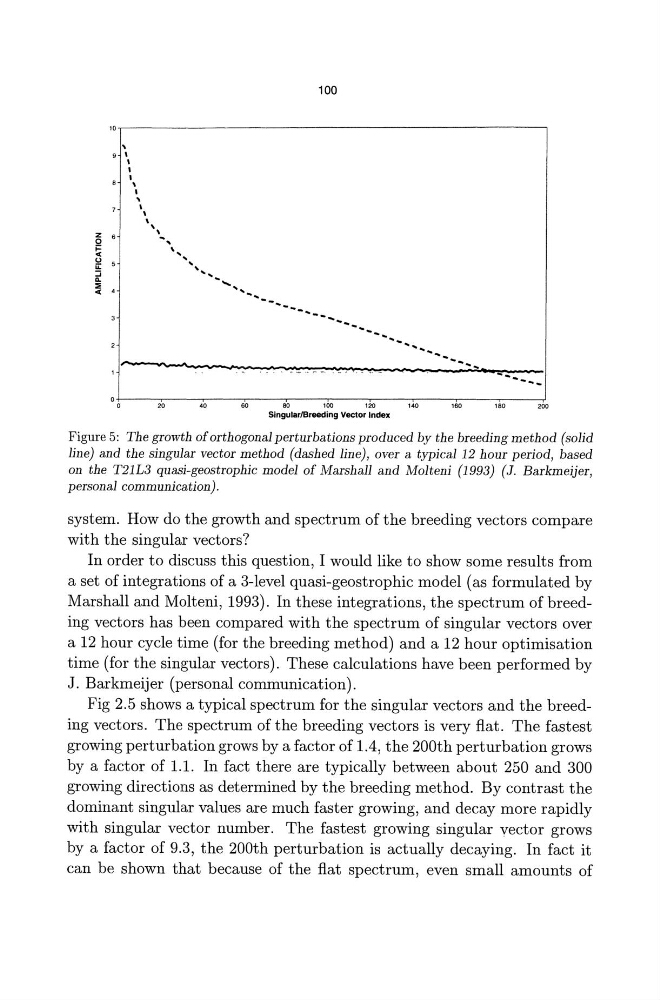
Figure 5: The growth of orthogonal perturbations produced by the breeding method (solid
line) and the singular vector method (dashed line), over a typical 12 hour period, based
on the T21L3 quasi-geostrophic model of Marshall and Molteni (1993) (J. Barkmeijer,
personal communication).
system. How do the growth and spectrum of the breeding vectors compare
with the singular vectors?
In order to discuss this question, I would like to show some results from
a set of integrations of a 3-level quasi-geostrophic model (as formulated by
Marshall and Molteni, 1993). In these integrations, the spectrum of breeding vectors has been compared with the spectrum of singular vectors over
a 12 hour cycle time (for the breeding method) and a 12 hour optimisation
time (for the singular vectors). These calculations have been performed by
J. Barkmeijer (personal communication).
Fig 2.5 shows a typical spectrum for the singular vectors and the breeding vectors. The spectrum of the breeding vectors is very flat. The fastest
growing perturbation grows by a factor of 1.4, the 200th perturbation grows
by a factor of 1.1. In fact there are typically between about 250 and 300
growing directions as determined by the breeding method. By contrast the
dominant singular values are much faster growing, and decay more rapidly
with singular vector number. The fastest growing singular vector grows
by a factor of 9.3, the 200th perturbation is actually decaying. In fact it
can be shown that because of the flat spectrum, even small amounts of
10,--------------------------------------------------,
,
9 ,
, , , , , , , , ,
"
o~--~----~--~----~--~~--~--~~--~----~--~
o
20
40
60
80
100
120
140
160
180
200
SingularlBreeding Vector Index
Figure 5: The growth of orthogonal perturbations produced by the breeding method (solid
line) and the singular vector method (dashed line), over a typical 12 hour period, based
on the T21L3 quasi-geostrophic model of Marshall and Molteni (1993) (J. Barkmeijer,
personal communication).
system. How do the growth and spectrum of the breeding vectors compare
with the singular vectors?
In order to discuss this question, I would like to show some results from
a set of integrations of a 3-level quasi-geostrophic model (as formulated by
Marshall and Molteni, 1993). In these integrations, the spectrum of breeding vectors has been compared with the spectrum of singular vectors over
a 12 hour cycle time (for the breeding method) and a 12 hour optimisation
time (for the singular vectors). These calculations have been performed by
J. Barkmeijer (personal communication).
Fig 2.5 shows a typical spectrum for the singular vectors and the breeding vectors. The spectrum of the breeding vectors is very flat. The fastest
growing perturbation grows by a factor of 1.4, the 200th perturbation grows
by a factor of 1.1. In fact there are typically between about 250 and 300
growing directions as determined by the breeding method. By contrast the
dominant singular values are much faster growing, and decay more rapidly
with singular vector number. The fastest growing singular vector grows
by a factor of 9.3, the 200th perturbation is actually decaying. In fact it
can be shown that because of the flat spectrum, even small amounts of