

97
(2.20)
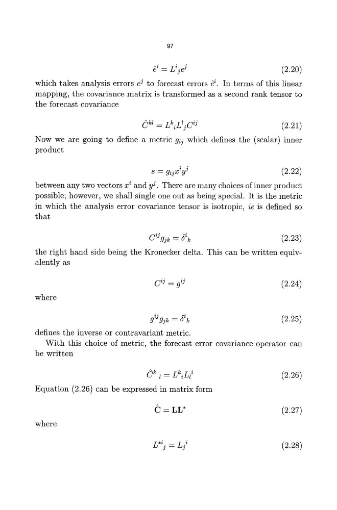
which takes analysis errors e j to forecast errors iii. In terms of this linear
mapping, the covariance matrix is transformed as a second rank tensor to
the forecast covariance
(2.21 )
Now we are going to define a metric gij which defines the (scalar) inner
product
(2.22)
between any two vectors xi and yj. There are many choices of inner product
possible; however, we shall single one out as being special. It is the metric
in which the analysis error covariance tensor is isotropic, ie is defined so
that
(2.23)
the right hand side being the Kronecker delta. This can be written equivalentlyas
where
gij9jk = 6 i k
defines the inverse or contravariant metric.
(2.24)
(2.25)
With this choice of metric, the forecast error covariance operator can
be written
~ k
k
i
C I=L iLl
Equation (2.26) can be expressed in matrix form
where
C =LL*
L *i. - L.i
J -
J
(2.26)
(2.27)
(2.28)
(2.20)
which takes analysis errors e j to forecast errors iii. In terms of this linear
mapping, the covariance matrix is transformed as a second rank tensor to
the forecast covariance
(2.21 )
Now we are going to define a metric gij which defines the (scalar) inner
product
(2.22)
between any two vectors xi and yj. There are many choices of inner product
possible; however, we shall single one out as being special. It is the metric
in which the analysis error covariance tensor is isotropic, ie is defined so
that
(2.23)
the right hand side being the Kronecker delta. This can be written equivalentlyas
where
gij9jk = 6 i k
defines the inverse or contravariant metric.
(2.24)
(2.25)
With this choice of metric, the forecast error covariance operator can
be written
~ k
k
i
C I=L iLl
Equation (2.26) can be expressed in matrix form
where
C =LL*
L *i. - L.i
J -
J
(2.26)
(2.27)
(2.28)