

93
10
30
a)
>b)
>~ 25 I
::I:
a: 20
~
0W
II
0
5
z 15 II
a:
w 10
1\
I-I
I
UJ
5.~
z
ex
w 0
Io '
0
0 5 10 15 20 25 30 35 40
I0 5 1 0 15 20 25 30 35 40
N WAVE NUMBER
N WAVE NUMBER
>10
~
c)
a:
w 5
z W
-I
ex
I0
0
0 5 10 15 20 25 30 35 40
lN WAVE NUMBER
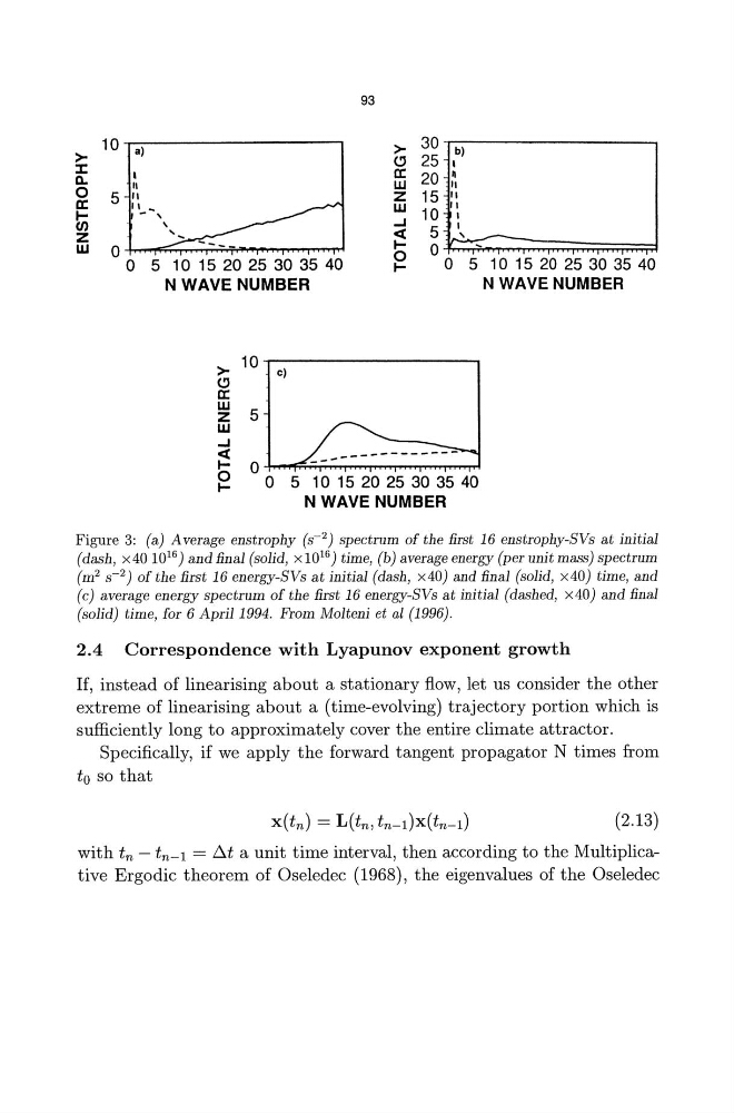
Figure 3: (a) Average enstrophy (S-2) spectrum of the first 16 enstrophy-SVs at initial
(dash, x40 10 16 ) and final (solid, x 10 16 ) time, (b) average energy (per unit mass) spectrum
(m 2 S-2) of the first 16 energy-SVs at initial (dash, x40) and final (solid, x40) time, and
(c) average energy spectrum of the first 16 energy-SVs at initial (dashed, x40) and final
(solid) time, for 6 April 1994. From Molteni et al (1996).
2.4 Correspondence with Lyapunov exponent growth
If, instead of linearising about a stationary flow, let us consider the other
extreme of linearising about a (time-evolving) trajectory portion which is
sufficiently long to approximately cover the entire climate attract or.
Specifically, if we apply the forward tangent propagator N times from
to so that
(2.13)
with tn - tn-l = 6..t a unit time interval, then according to the Multiplicative Ergodic theorem of Oseledec (1968), the eigenvalues of the Oseledec
10
30
a)
>b)
>~ 25 I
::I:
a: 20
~
0W
II
0
5
z 15 II
a:
w 10
1\
I-I
I
UJ
5.~
z
ex
w 0
Io '
0
0 5 10 15 20 25 30 35 40
I0 5 1 0 15 20 25 30 35 40
N WAVE NUMBER
N WAVE NUMBER
>10
~
c)
a:
w 5
z W
-I
ex
I0
0
0 5 10 15 20 25 30 35 40
lN WAVE NUMBER
Figure 3: (a) Average enstrophy (S-2) spectrum of the first 16 enstrophy-SVs at initial
(dash, x40 10 16 ) and final (solid, x 10 16 ) time, (b) average energy (per unit mass) spectrum
(m 2 S-2) of the first 16 energy-SVs at initial (dash, x40) and final (solid, x40) time, and
(c) average energy spectrum of the first 16 energy-SVs at initial (dashed, x40) and final
(solid) time, for 6 April 1994. From Molteni et al (1996).
2.4 Correspondence with Lyapunov exponent growth
If, instead of linearising about a stationary flow, let us consider the other
extreme of linearising about a (time-evolving) trajectory portion which is
sufficiently long to approximately cover the entire climate attract or.
Specifically, if we apply the forward tangent propagator N times from
to so that
(2.13)
with tn - tn-l = 6..t a unit time interval, then according to the Multiplicative Ergodic theorem of Oseledec (1968), the eigenvalues of the Oseledec