

CHAPTER 8 ' Physical Characteristics and Processes of the Rio de la Plata Estuary
-34.5
cp - 35.0
"'C
::J
::
iii
...J -35.5
-36.0
-58.0
-57.5
-+ 0.5 ms- 1
p
-
~
~
-
-
~
-
,
,
r
r
_
_
_
_
_
_
~
~
r
r
_
_
_
_
_
;
~
~
- - - - - -
, ~ ~ ~ - - - - -
~
~
y
.~
-
-
-
-
"
. '
,1
~~
~~
~~
_~
_~
~r
_ _ _ _ _ _ _ _
~
•
-
~
~
~
v
~
~
~
~
~
~
_
,
-
-
_
~
~
_
~
_
.r
_
_
_
,
~
_
r
~
r
r
_
_
~
~
_
_
~
~
~
_
_
_
_
_
_
~
r
_
_
\
~
~
~
~
~
~
_
~
~
r
r
_
,
~
~
~
_
_
~
~
~
r
r
_
\
~ ~ ~ ~ ~ ~ - ~ ~ - - ~
~ ~ ~ ~ ~ ~ ~ ~ ~ ~ ~ ~ =
,
~
~
~
~
,
~
~
~
_
_
r
,
~
~
~
~
~
_
~
~
r
~
_
,
~
~
~
~
~
~
~
~
_
r
_
': ~::~::~~~~ ... : ': .. :-:
..... <-(-~.');. ' "
............ ' , -
_ . . . . .
-56.5
- 56.0
- 55.5
Longitude
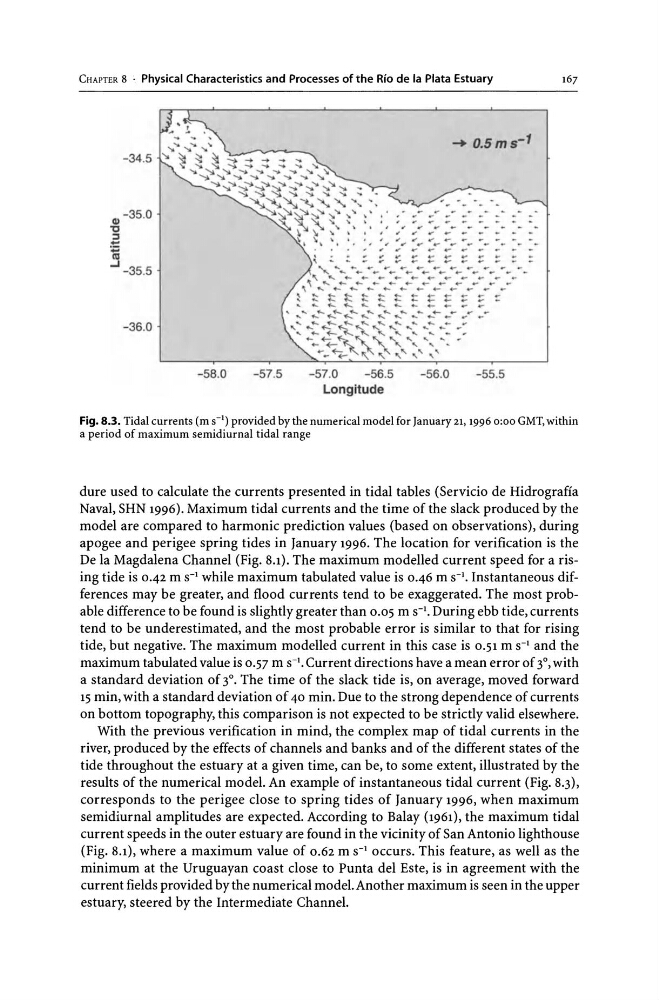
Fig. 8.3. Tidal currents (m S-I) provided by the numerical model for January 21,19960:00 GMT, within
a period of maximum semidiurnal tidal range
dure used to calculate the currents presented in tidal tables (Servicio de Hidrografia
Naval, SHN 1996). Maximum tidal currents and the time of the slack produced by the
model are compared to harmonic prediction values (based on observations), during
apogee and perigee spring tides in January 1996. The location for verification is the
De la Magdalena Channel (Fig. 8.1). The maximum modelled current speed for a rising tide is 0.42 m S-1 while maximum tabulated value is 0.46 m S-I. Instantaneous differences may be greater, and flood currents tend to be exaggerated. The most probable difference to be found is slightly greater than 0.05 m S-I. During ebb tide, currents
tend to be underestimated, and the most probable error is similar to that for rising
tide, but negative. The maximum modelled current in this case is 0.51 m S-1 and the
maximum tabulated value is 0.57 m S-I. Current directions have a mean error of 3°, with
a standard deviation of 3°. The time of the slack tide is, on average, moved forward
15 min, with a standard deviation of 40 min. Due to the strong dependence of currents
on bottom topography, this comparison is not expected to be strictly valid elsewhere.
With the previous verification in mind, the complex map of tidal currents in the
river, produced by the effects of channels and banks and of the different states of the
tide throughout the estuary at a given time, can be, to some extent, illustrated by the
results of the numerical model. An example of instantaneous tidal current (Fig. 8.3),
corresponds to the perigee close to spring tides of January 1996, when maximum
semidiurnal amplitudes are expected. According to Balay (1961), the maximum tidal
current speeds in the outer estuary are found in the vicinity of San Antonio lighthouse
(Fig. 8.1), where a maximum value of 0.62 m S-1 occurs. This feature, as well as the
minimum at the Uruguayan coast close to Punta del Este, is in agreement with the
current fields provided by the numerical model. Another maximum is seen in the upper
estuary, steered by the Intermediate Channel.
-34.5
cp - 35.0
"'C
::J
::
iii
...J -35.5
-36.0
-58.0
-57.5
-+ 0.5 ms- 1
p
-
~
~
-
-
~
-
,
,
r
r
_
_
_
_
_
_
~
~
r
r
_
_
_
_
_
;
~
~
- - - - - -
, ~ ~ ~ - - - - -
~
~
y
.~
-
-
-
-
"
. '
,1
~~
~~
~~
_~
_~
~r
_ _ _ _ _ _ _ _
~
•
-
~
~
~
v
~
~
~
~
~
~
_
,
-
-
_
~
~
_
~
_
.r
_
_
_
,
~
_
r
~
r
r
_
_
~
~
_
_
~
~
~
_
_
_
_
_
_
~
r
_
_
\
~
~
~
~
~
~
_
~
~
r
r
_
,
~
~
~
_
_
~
~
~
r
r
_
\
~ ~ ~ ~ ~ ~ - ~ ~ - - ~
~ ~ ~ ~ ~ ~ ~ ~ ~ ~ ~ ~ =
,
~
~
~
~
,
~
~
~
_
_
r
,
~
~
~
~
~
_
~
~
r
~
_
,
~
~
~
~
~
~
~
~
_
r
_
': ~::~::~~~~ ... : ': .. :-:
..... <-(-~.');. ' "
............ ' , -
_ . . . . .
-56.5
- 56.0
- 55.5
Longitude
Fig. 8.3. Tidal currents (m S-I) provided by the numerical model for January 21,19960:00 GMT, within
a period of maximum semidiurnal tidal range
dure used to calculate the currents presented in tidal tables (Servicio de Hidrografia
Naval, SHN 1996). Maximum tidal currents and the time of the slack produced by the
model are compared to harmonic prediction values (based on observations), during
apogee and perigee spring tides in January 1996. The location for verification is the
De la Magdalena Channel (Fig. 8.1). The maximum modelled current speed for a rising tide is 0.42 m S-1 while maximum tabulated value is 0.46 m S-I. Instantaneous differences may be greater, and flood currents tend to be exaggerated. The most probable difference to be found is slightly greater than 0.05 m S-I. During ebb tide, currents
tend to be underestimated, and the most probable error is similar to that for rising
tide, but negative. The maximum modelled current in this case is 0.51 m S-1 and the
maximum tabulated value is 0.57 m S-I. Current directions have a mean error of 3°, with
a standard deviation of 3°. The time of the slack tide is, on average, moved forward
15 min, with a standard deviation of 40 min. Due to the strong dependence of currents
on bottom topography, this comparison is not expected to be strictly valid elsewhere.
With the previous verification in mind, the complex map of tidal currents in the
river, produced by the effects of channels and banks and of the different states of the
tide throughout the estuary at a given time, can be, to some extent, illustrated by the
results of the numerical model. An example of instantaneous tidal current (Fig. 8.3),
corresponds to the perigee close to spring tides of January 1996, when maximum
semidiurnal amplitudes are expected. According to Balay (1961), the maximum tidal
current speeds in the outer estuary are found in the vicinity of San Antonio lighthouse
(Fig. 8.1), where a maximum value of 0.62 m S-1 occurs. This feature, as well as the
minimum at the Uruguayan coast close to Punta del Este, is in agreement with the
current fields provided by the numerical model. Another maximum is seen in the upper
estuary, steered by the Intermediate Channel.