

2.5 Basic Analytical Properties
67
The sensitivity is the slope of the central linear portion of the curve. A sample
that contains no analyte (an analytical blank) produces an analytical signal XB
due to both the sample matrix and the instrument's background noise that is
called a "blank signal".
The calibration curve consists of three distinct portions as regards sensitivity,
namely:
(a) At low analyte concentrations (5 = 0), the analyte cannot be detected or
determined. The signal, XB' is produced by the blank and coincides with the
intercept. If the blank gives no signal, then the curve intersects the origin
(x= 0, C= 0).
(b) At intermediate analyte concentrations, the sensitivity is non-zero (5) 0). In
this case, a dynamic range is bounded the lower limit of which is the limit of
detection. This range comprises three sub-zones. In the central one, 5 remains
constant; this is the so-called "linear range", which is bounded by the other
two regions (where 5 decreases and increases, respectively). The lower limit
of the linear range defines the coordinates for the limit of quantitation. The
upper limit of the linear range is reached when the deviation from linearity
(x'-x") equals or exceeds 0.03 times x' (the value where linearity starts); if
the deviation is greater, then the curve falls outside the linear range.
(c) At very high analyte concentrations, the signal no longer varies with the
concentration (5 = 0) and the curve is parallel to the initial portion - at a
higher signal level, however.
The quantitative definition of sensitivity is completed by several parameters that
establish the minimum concentrations that can be detected or determined. Thus,
the limit of detection is the analyte concentration CWD which produces a signal XWD
that can be statistically distinguished from the blank signal. This parameter is quantified in preliminary experiments involving measuring n blanks to obtain a mean
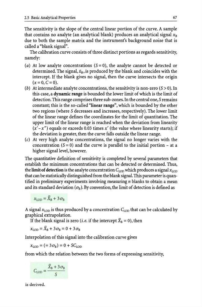
and its standard deviation (OB). By convention, the limit of detection is defined as
XWD = XB + 30B
A signal XWD is thus produced by a concentration CWD that can be calculated by
graphical extrapolation.
If the blank signal is zero (i. e. if the intercept XB = 0), then
XWD = XB + 30B = 0 + 30B
Interpolation of this signal into the calibration curve gives
XWD = (= 3oB) = 0 + 5CWD
from which the relation between the two forms of expressing sensitivity,
XB +3UB
C WD = - - -
5
is derived.
67
The sensitivity is the slope of the central linear portion of the curve. A sample
that contains no analyte (an analytical blank) produces an analytical signal XB
due to both the sample matrix and the instrument's background noise that is
called a "blank signal".
The calibration curve consists of three distinct portions as regards sensitivity,
namely:
(a) At low analyte concentrations (5 = 0), the analyte cannot be detected or
determined. The signal, XB' is produced by the blank and coincides with the
intercept. If the blank gives no signal, then the curve intersects the origin
(x= 0, C= 0).
(b) At intermediate analyte concentrations, the sensitivity is non-zero (5) 0). In
this case, a dynamic range is bounded the lower limit of which is the limit of
detection. This range comprises three sub-zones. In the central one, 5 remains
constant; this is the so-called "linear range", which is bounded by the other
two regions (where 5 decreases and increases, respectively). The lower limit
of the linear range defines the coordinates for the limit of quantitation. The
upper limit of the linear range is reached when the deviation from linearity
(x'-x") equals or exceeds 0.03 times x' (the value where linearity starts); if
the deviation is greater, then the curve falls outside the linear range.
(c) At very high analyte concentrations, the signal no longer varies with the
concentration (5 = 0) and the curve is parallel to the initial portion - at a
higher signal level, however.
The quantitative definition of sensitivity is completed by several parameters that
establish the minimum concentrations that can be detected or determined. Thus,
the limit of detection is the analyte concentration CWD which produces a signal XWD
that can be statistically distinguished from the blank signal. This parameter is quantified in preliminary experiments involving measuring n blanks to obtain a mean
and its standard deviation (OB). By convention, the limit of detection is defined as
XWD = XB + 30B
A signal XWD is thus produced by a concentration CWD that can be calculated by
graphical extrapolation.
If the blank signal is zero (i. e. if the intercept XB = 0), then
XWD = XB + 30B = 0 + 30B
Interpolation of this signal into the calibration curve gives
XWD = (= 3oB) = 0 + 5CWD
from which the relation between the two forms of expressing sensitivity,
XB +3UB
C WD = - - -
5
is derived.