66
2 Analytical Properties
The most widely accepted form of expressing sensitivity, S, is the "variation of
the analytical signal, x, with the analyte concentration, e", which can be expressed in absolute, differential or incremental terms:
x
6x 6x
S= -
S=-=C
6C 6C
The first part of the definition only holds if the signal is exclusively due to the
presence of the analyte, i. e. in the absence of spurious signals called "analytical
blanks" (C = 0). The more marked the change in the signal produced by a small
change in the analyte concentration is, the higher will be the sensitivity. This idea
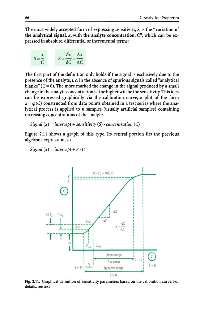
can be expressed graphically via the calibration curve, a plot of the form
x = increasing concentrations of the analyte.
Signal (x) = intercept + sensitivity (S) . concentration (C)
Figure 2.11 shows a graph of this type. Its central portion fits the previous
algebraic expression, so
Signal (x) = intercept + S . C
x'
x"
I
I
I I
I I I
I I I
(x'·x") = 0.Q3 x'
c
I 1 I
x
x
5=tJ.C
I ( lOO 1 CLOQ
l~~~ __________ ~--I
I
linear range
I
I
I
I
I
I +~ ____________ ~
I
I
5 = conSI
-, 5--> 0 I
I
5 I
I
,
Dynam ic range
I
5 = 0 : "'~.,.,
I ~~--------------------+ _I
5>0
0
5=0
Fig.2.11. Graphical definition of sensitivity parameters based on the calibration curve. For
details, see text