

6.3 Relative Quantitation Methods
273
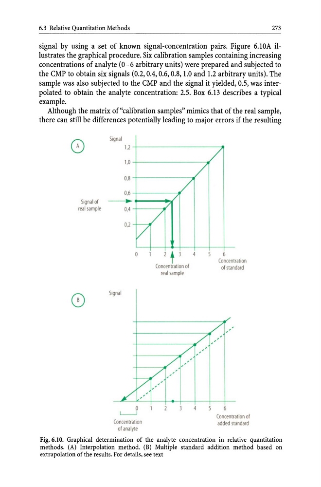
signal by using a set of known signal-concentration pairs. Figure 6.lOA illustrates the graphical procedure. Six calibration samples containing increasing
concentrations of analyte (0-6 arbitrary units) were prepared and subjected to
the CMP to obtain six signals (0.2,0.4,0.6,0.8,1.0 and 1.2 arbitrary units). The
sample was also subjected to the CMP and the signal it yielded, 0.5, was interpolated to obtain the analyte concentration: 2.5. Box 6.13 describes a typical
example.
Although the matrix of "calibration samples" mimics that of the real sample,
there can still be differences potentially leading to major errors if the resulting
0
Signal of
real sample
Signal
1.2
1,0
0,8
0,6
•
/
/
/
/
0,4
0.2
-7 /
o
Signal
o
L-..J
Concentration
of analyte
2 t 3
Concentration of
real sample
2
4
4
/
6
Concentration
of standard
5
6
Concentra tion of
added standard
Fig. 6.10. Graphical determination of the analyte concentration in relative quantitation
methods. (A) Interpolation method. (B) Multiple standard addition method based on
extrapolation of the results. For details, see text
273
signal by using a set of known signal-concentration pairs. Figure 6.lOA illustrates the graphical procedure. Six calibration samples containing increasing
concentrations of analyte (0-6 arbitrary units) were prepared and subjected to
the CMP to obtain six signals (0.2,0.4,0.6,0.8,1.0 and 1.2 arbitrary units). The
sample was also subjected to the CMP and the signal it yielded, 0.5, was interpolated to obtain the analyte concentration: 2.5. Box 6.13 describes a typical
example.
Although the matrix of "calibration samples" mimics that of the real sample,
there can still be differences potentially leading to major errors if the resulting
0
Signal of
real sample
Signal
1.2
1,0
0,8
0,6
•
/
/
/
/
0,4
0.2
-7 /
o
Signal
o
L-..J
Concentration
of analyte
2 t 3
Concentration of
real sample
2
4
4
/
6
Concentration
of standard
5
6
Concentra tion of
added standard
Fig. 6.10. Graphical determination of the analyte concentration in relative quantitation
methods. (A) Interpolation method. (B) Multiple standard addition method based on
extrapolation of the results. For details, see text