

CHAPTER 21 . (hemometries for Sampling and Analysis: Theory and Environmental Applications
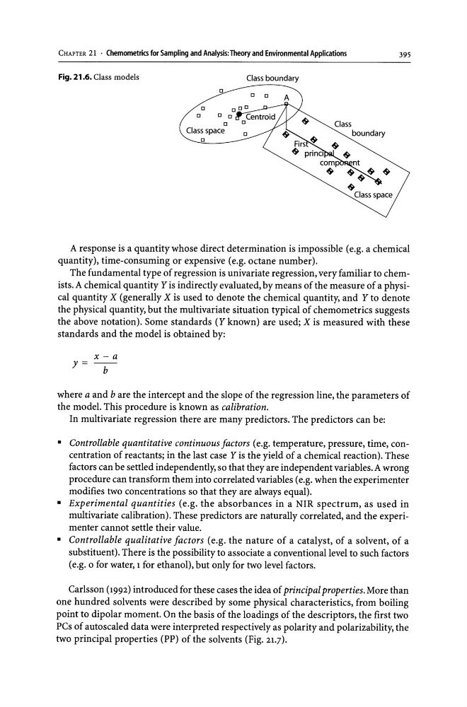
Fig. 21.6. Class models
o
o
o
o
Class space
o
Class boundary
o
Class
boundary
395
A response is a quantity whose direct determination is impossible (e.g. a chemical
quantity), time-consuming or expensive (e.g. octane number).
The fundamental type of regression is univariate regression, very familiar to chemists. A chemical quantity Y is indirectly evaluated, by means of the measure of a physical quantity X (generally X is used to denote the chemical quantity, and Y to denote
the physical quantity, but the multivariate situation typical of chemometrics suggests
the above notation). Some standards (Y known) are used; X is measured with these
standards and the model is obtained by:
x-a
y=
b
where a and b are the intercept and the slope of the regression line, the parameters of
the model. This procedure is known as calibration.
In multivariate regression there are many predictors. The predictors can be:
• Controllable quantitative continuous factors (e.g. temperature, pressure, time, concentration of reactants; in the last case Y is the yield of a chemical reaction). These
factors can be settled independently, so that they are independent variables. A wrong
procedure can transform them into correlated variables (e.g. when the experimenter
modifies two concentrations so that they are always equal) .
• Experimental quantities (e.g. the absorbances in a NIR spectrum, as used in
multivariate calibration). These predictors are naturally correlated, and the experimenter cannot settle their value.
• Controllable qualitative factors (e.g. the nature of a catalyst, of a solvent, of a
substituent). There is the possibility to associate a conventional level to such factors
(e.g. 0 for water, 1 for ethanol), but only for two level factors.
Carlsson (1992) introduced for these cases the idea of principal properties. More than
one hundred solvents were described by some physical characteristics, from boiling
point to dipolar moment. On the basis of the loadings of the descriptors, the first two
PCs of auto scaled data were interpreted respectively as polarity and polarizability, the
two principal properties (PP) of the solvents (Fig. 21.7).
Fig. 21.6. Class models
o
o
o
o
Class space
o
Class boundary
o
Class
boundary
395
A response is a quantity whose direct determination is impossible (e.g. a chemical
quantity), time-consuming or expensive (e.g. octane number).
The fundamental type of regression is univariate regression, very familiar to chemists. A chemical quantity Y is indirectly evaluated, by means of the measure of a physical quantity X (generally X is used to denote the chemical quantity, and Y to denote
the physical quantity, but the multivariate situation typical of chemometrics suggests
the above notation). Some standards (Y known) are used; X is measured with these
standards and the model is obtained by:
x-a
y=
b
where a and b are the intercept and the slope of the regression line, the parameters of
the model. This procedure is known as calibration.
In multivariate regression there are many predictors. The predictors can be:
• Controllable quantitative continuous factors (e.g. temperature, pressure, time, concentration of reactants; in the last case Y is the yield of a chemical reaction). These
factors can be settled independently, so that they are independent variables. A wrong
procedure can transform them into correlated variables (e.g. when the experimenter
modifies two concentrations so that they are always equal) .
• Experimental quantities (e.g. the absorbances in a NIR spectrum, as used in
multivariate calibration). These predictors are naturally correlated, and the experimenter cannot settle their value.
• Controllable qualitative factors (e.g. the nature of a catalyst, of a solvent, of a
substituent). There is the possibility to associate a conventional level to such factors
(e.g. 0 for water, 1 for ethanol), but only for two level factors.
Carlsson (1992) introduced for these cases the idea of principal properties. More than
one hundred solvents were described by some physical characteristics, from boiling
point to dipolar moment. On the basis of the loadings of the descriptors, the first two
PCs of auto scaled data were interpreted respectively as polarity and polarizability, the
two principal properties (PP) of the solvents (Fig. 21.7).