

3.11 Example
63
%
* e,
4th order CDS
-r
. .
2nd order CDS
. '% . .. . .
3
0.0
0.2
0.4
0.6
0.8
1.0
.*
4lh order CDS
. .
. .
. .
2nd order CDS
. '% . .. . .
3
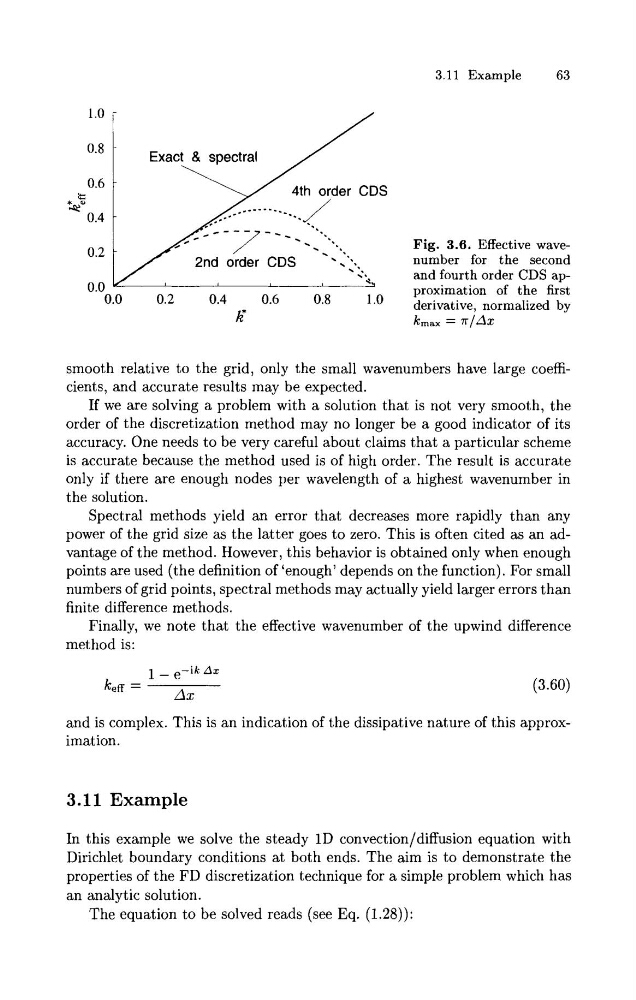
Fig. 3.6. Effective wavenumber for the second
and fourth order CDS approximation of the first
derivative, normalized by
smooth relative to the grid, only the small wavenumbers have large coefficients, and accurate results may be expected.
If we are solving a problem with a solution that is not very smooth, the
order of the discretization method may no longer be a good indicator of its
accuracy. One needs to be very careful about claims that a particular scheme
is accurate because the method used is of high order. The result is accurate
only if there are enough nodes per wavelength of a highest wavenumber in
the solution.
Spectral methods yield an error that decreases more rapidly than any
power of the grid size as the latter goes to zero. This is often cited as an advantage of the method. However, this behavior is obtained only when enough
points are used (the definition of 'enough' depends on the function). For small
numbers of grid points, spectral methods may actually yield larger errors than
finite difference methods.
Finally, we note that the effective wavenumber of the upwind difference
method is:
and is complex. This is an indication of the dissipative nature of this approximation.
3.1 1 Example
In this example we solve the steady 1D convection/diffusion equation with
Dirichlet boundary conditions at both ends. The aim is to demonstrate the
properties of the FD discretization technique for a simple problem which has
an analytic solution.
The equation to be solved reads (see Eq. (1.28)):
63
%
* e,
4th order CDS
-r
. .
2nd order CDS
. '% . .. . .
3
0.0
0.2
0.4
0.6
0.8
1.0
.*
4lh order CDS
. .
. .
. .
2nd order CDS
. '% . .. . .
3
Fig. 3.6. Effective wavenumber for the second
and fourth order CDS approximation of the first
derivative, normalized by
smooth relative to the grid, only the small wavenumbers have large coefficients, and accurate results may be expected.
If we are solving a problem with a solution that is not very smooth, the
order of the discretization method may no longer be a good indicator of its
accuracy. One needs to be very careful about claims that a particular scheme
is accurate because the method used is of high order. The result is accurate
only if there are enough nodes per wavelength of a highest wavenumber in
the solution.
Spectral methods yield an error that decreases more rapidly than any
power of the grid size as the latter goes to zero. This is often cited as an advantage of the method. However, this behavior is obtained only when enough
points are used (the definition of 'enough' depends on the function). For small
numbers of grid points, spectral methods may actually yield larger errors than
finite difference methods.
Finally, we note that the effective wavenumber of the upwind difference
method is:
and is complex. This is an indication of the dissipative nature of this approximation.
3.1 1 Example
In this example we solve the steady 1D convection/diffusion equation with
Dirichlet boundary conditions at both ends. The aim is to demonstrate the
properties of the FD discretization technique for a simple problem which has
an analytic solution.
The equation to be solved reads (see Eq. (1.28)):