

12.4 Moving Grids
375
Conservation equations for scalar quantities are easily derived from the corresponding equations for a fixed CV by replacing the velocity vector in the
convective term with the relative velocity v - vb.
Obviously, if the boundary moves with the same velocity as the fluid, the
mass flux through the CV face will be zero. If this is true for all CV faces,
then the same fluid remains within the CV and it becomes a control mass;
we then have the Lagrangian description of fluid motion. On the other hand,
if the CV does not move, the equations are those dealt with earlier.
When the location of the grid is known as a function of time, solution of
the Navier-Stokes equations poses no new problems: we simply calculate the
convective fluxes (e.g. the mass fluxes) using the relative velocity components
at the cell faces. However, when the cell faces move, conservation of mass (and
all other conserved quantities) is not necessarily ensured if the grid velocities
are used to calculate the mass fluxes. For example, consider the continuity
equation with implicit Euler time integration; for the sake of simplicity we
assume that the CV is rectangular and that the fluid is incompressible and
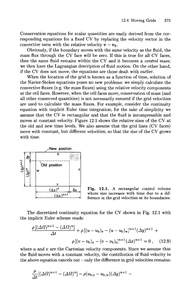
moves at constant velocity. Figure 12.1 shows the relative sizes of the CV a t
the old and new time levels. We also assume that the grid lines (CV faces)
move with constant, but different velocities, so that the size of the CV grows
with time.
,New position
Fig. 12.1. A rectangular control volume
whose size increases with time due to a difference in the grid velocities at its boundaries.
The discretized continuity equation for the CV shown in Fig. 12.1 with
the implicit Euler scheme reads:
p [(v - v ~ ) ~
- (2, - V ~ ) ~ ] ~ + ~ ( A X ) ~ + '
= 0 , (12.9)
where u and v are the Cartesian velocity components. Since we assume that
the fluid moves with a constant velocity, the contribution of fluid velocity in
the above equation cancels out -only the difference in grid velocities remains:
375
Conservation equations for scalar quantities are easily derived from the corresponding equations for a fixed CV by replacing the velocity vector in the
convective term with the relative velocity v - vb.
Obviously, if the boundary moves with the same velocity as the fluid, the
mass flux through the CV face will be zero. If this is true for all CV faces,
then the same fluid remains within the CV and it becomes a control mass;
we then have the Lagrangian description of fluid motion. On the other hand,
if the CV does not move, the equations are those dealt with earlier.
When the location of the grid is known as a function of time, solution of
the Navier-Stokes equations poses no new problems: we simply calculate the
convective fluxes (e.g. the mass fluxes) using the relative velocity components
at the cell faces. However, when the cell faces move, conservation of mass (and
all other conserved quantities) is not necessarily ensured if the grid velocities
are used to calculate the mass fluxes. For example, consider the continuity
equation with implicit Euler time integration; for the sake of simplicity we
assume that the CV is rectangular and that the fluid is incompressible and
moves at constant velocity. Figure 12.1 shows the relative sizes of the CV a t
the old and new time levels. We also assume that the grid lines (CV faces)
move with constant, but different velocities, so that the size of the CV grows
with time.
,New position
Fig. 12.1. A rectangular control volume
whose size increases with time due to a difference in the grid velocities at its boundaries.
The discretized continuity equation for the CV shown in Fig. 12.1 with
the implicit Euler scheme reads:
p [(v - v ~ ) ~
- (2, - V ~ ) ~ ] ~ + ~ ( A X ) ~ + '
= 0 , (12.9)
where u and v are the Cartesian velocity components. Since we assume that
the fluid moves with a constant velocity, the contribution of fluid velocity in
the above equation cancels out -only the difference in grid velocities remains: