

11.4 Adaptive Grid Methods and Local Grid Refinement
353
difference between fluxes computed using the cubic ( F: )
and linear fits ( F f )
should be added to the discretized equation as an additional source term to
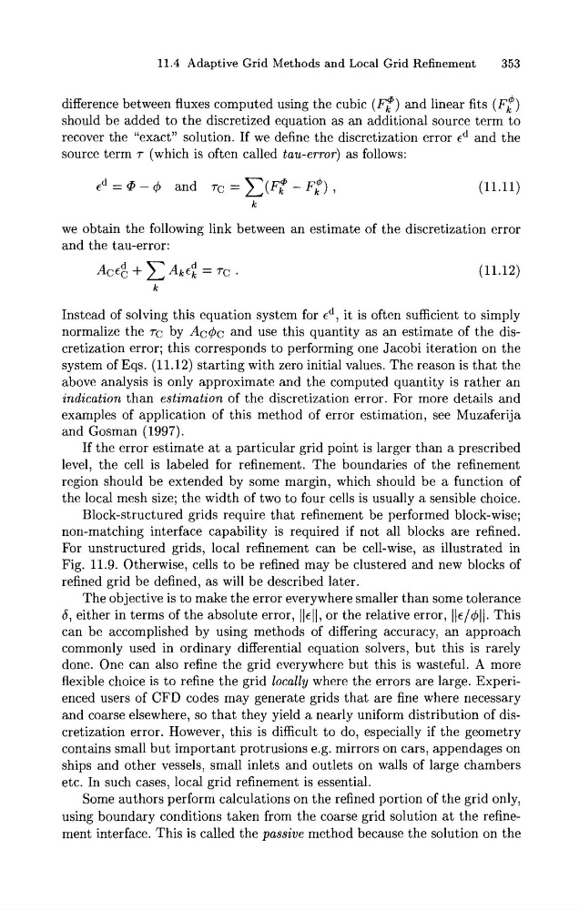
recover the "exact" solution. If we define the discretization error td and the
source term T (which is often called tau-error) as follows:
td = @ - q 5
and TC = C(F: - F f ) ,
k
we obtain the following link between an estimate of the discretization error
and the tau-error:
Instead of solving this equation system for t d , it is often sufficient to simply
normalize the TC by Acq5c and use this quantity as an estimate of the discretization error; this corresponds to performing one Jacobi iteration on the
system of Eqs. (11.12) starting with zero initial values. The reason is that the
above analysis is only approximate and the computed quantity is rather an
indication than estimation of the discretization error. For more details and
examples of application of this method of error estimation, see Muzaferija
and Gosman (1997).
If the error estimate at a particular grid point is larger than a prescribed
level, the cell is labeled for refinement. The boundaries of the refinement
region should be extended by some margin, which should be a function of
the local mesh size; the width of two to four cells is usually a sensible choice.
Block-structured grids require that refinement be performed block-wise;
non-matching interface capability is required if not all blocks are refined.
For unstructured grids, local refinement can be cell-wise, as illustrated in
Fig. 11.9. Otherwise, cells to be refined may be clustered and new blocks of
refined grid be defined, as will be described later.
The objective is to make the error everywhere smaller than some tolerance
6, either in terms of the absolute error, IIcII, or the relative error, IIc/~II. This
can be accomplished by using methods of differing accuracy, an approach
commonly used in ordinary differential equation solvers, but this is rarely
done. One can also refine the grid everywhere but this is wasteful. A more
flexible choice is to refine the grid locally where the errors are large. Experienced users of CFD codes may generate grids that are fine where necessary
and coarse elsewhere, so that they yield a nearly uniform distribution of discretization error. However, this is difficult to do, especially if the geometry
contains small but important protrusions e.g. mirrors on cars, appendages on
ships and other vessels, small inlets and outlets on walls of large chambers
etc. In such cases, local grid refinement is essential.
Some authors perform calculations on the refined portion of the grid only,
using boundary conditions taken from the coarse grid solution at the refinement interface. This is called the passive method because the solution on the
353
difference between fluxes computed using the cubic ( F: )
and linear fits ( F f )
should be added to the discretized equation as an additional source term to
recover the "exact" solution. If we define the discretization error td and the
source term T (which is often called tau-error) as follows:
td = @ - q 5
and TC = C(F: - F f ) ,
k
we obtain the following link between an estimate of the discretization error
and the tau-error:
Instead of solving this equation system for t d , it is often sufficient to simply
normalize the TC by Acq5c and use this quantity as an estimate of the discretization error; this corresponds to performing one Jacobi iteration on the
system of Eqs. (11.12) starting with zero initial values. The reason is that the
above analysis is only approximate and the computed quantity is rather an
indication than estimation of the discretization error. For more details and
examples of application of this method of error estimation, see Muzaferija
and Gosman (1997).
If the error estimate at a particular grid point is larger than a prescribed
level, the cell is labeled for refinement. The boundaries of the refinement
region should be extended by some margin, which should be a function of
the local mesh size; the width of two to four cells is usually a sensible choice.
Block-structured grids require that refinement be performed block-wise;
non-matching interface capability is required if not all blocks are refined.
For unstructured grids, local refinement can be cell-wise, as illustrated in
Fig. 11.9. Otherwise, cells to be refined may be clustered and new blocks of
refined grid be defined, as will be described later.
The objective is to make the error everywhere smaller than some tolerance
6, either in terms of the absolute error, IIcII, or the relative error, IIc/~II. This
can be accomplished by using methods of differing accuracy, an approach
commonly used in ordinary differential equation solvers, but this is rarely
done. One can also refine the grid everywhere but this is wasteful. A more
flexible choice is to refine the grid locally where the errors are large. Experienced users of CFD codes may generate grids that are fine where necessary
and coarse elsewhere, so that they yield a nearly uniform distribution of discretization error. However, this is difficult to do, especially if the geometry
contains small but important protrusions e.g. mirrors on cars, appendages on
ships and other vessels, small inlets and outlets on walls of large chambers
etc. In such cases, local grid refinement is essential.
Some authors perform calculations on the refined portion of the grid only,
using boundary conditions taken from the coarse grid solution at the refinement interface. This is called the passive method because the solution on the