

10.2 Pressure-Correction Methods for Arbitrary Mach Number
311
where T is the stress tensor (including pressure terms) and b represents body
forces per unit mass; see Chap. 1 for a discussion of various forms of these
equations.
It is natural to use the continuity equation to compute the density and to
derive the temperature from the energy equation. This leaves role of determining the pressure to the equation of state. We thus see that the roles of the
various equations are quite different from the ones they play in incompressible flows. Also note that the nature of the pressure is completely different.
In incompressible flows there is only the dynamic pressure whose absolute
value is of no consequence; for compressible flows, it is the thermodynamic
pressure whose absolute value is of critical importance.
The discretization of the equations can be carried out using the methods
described in Chaps. 3 and 4. The only changes required involve the boundary
conditions (which need to be different because the compressible equations are
hyperbolic in character), the nature and treatment of the coupling between
the density and the pressure, and the fact that shock waves, which are very
thin regions of extremely large change in many of the variables, may exist in
compressible flows. Below we shall extend the pressure-correction method to
flows at arbitrary Mach number, following the approach of DemirdiiC et al.
(1993). Similar methods have been published by Issa and Lockwood (1977),
Karki and Patankar (1989) and Van Doormal et al. (1987).
10.2.1 Pressure-Velocity-Density Coupling
As mentioned above, the discretization of the compressible momentum equations is essentially identical to that employed for the incompressible equations, see Chaps. 7 and 8, so we shall not repeat it here. We shall limit the
discussion to the implicit pressure-correction method described in Chap. 7,
but the ideas can be applied to other schemes as well.
To obtain the solution at the new time level, several outer iterations are
performed; see Sect. 7.3.4 for a detailed description of the scheme for incompressible flows. If time step is small, only a few outer iterations per time
step are necessary. For steady problems, the time step may be infinite and
the under-relaxation parameter acts like a pseudo-time step. We consider
only the segregated solution method, in which the linearized (around values
from the previous outer iteration) equations for velocity components, pressure correction, temperature and other scalar variables are solved in turn.
While solving for one variable, other variables are treated as known.
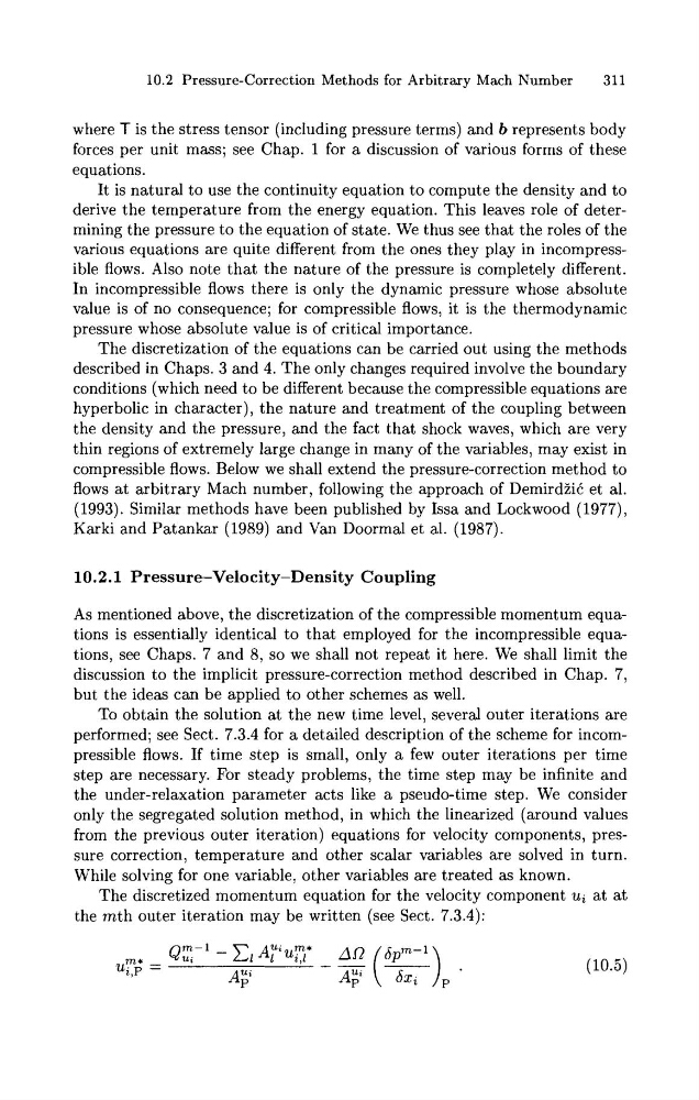
The discretized momentum equation for the velocity component ui at a t
the mth outer iteration may be written (see Sect. 7.3.4):
311
where T is the stress tensor (including pressure terms) and b represents body
forces per unit mass; see Chap. 1 for a discussion of various forms of these
equations.
It is natural to use the continuity equation to compute the density and to
derive the temperature from the energy equation. This leaves role of determining the pressure to the equation of state. We thus see that the roles of the
various equations are quite different from the ones they play in incompressible flows. Also note that the nature of the pressure is completely different.
In incompressible flows there is only the dynamic pressure whose absolute
value is of no consequence; for compressible flows, it is the thermodynamic
pressure whose absolute value is of critical importance.
The discretization of the equations can be carried out using the methods
described in Chaps. 3 and 4. The only changes required involve the boundary
conditions (which need to be different because the compressible equations are
hyperbolic in character), the nature and treatment of the coupling between
the density and the pressure, and the fact that shock waves, which are very
thin regions of extremely large change in many of the variables, may exist in
compressible flows. Below we shall extend the pressure-correction method to
flows at arbitrary Mach number, following the approach of DemirdiiC et al.
(1993). Similar methods have been published by Issa and Lockwood (1977),
Karki and Patankar (1989) and Van Doormal et al. (1987).
10.2.1 Pressure-Velocity-Density Coupling
As mentioned above, the discretization of the compressible momentum equations is essentially identical to that employed for the incompressible equations, see Chaps. 7 and 8, so we shall not repeat it here. We shall limit the
discussion to the implicit pressure-correction method described in Chap. 7,
but the ideas can be applied to other schemes as well.
To obtain the solution at the new time level, several outer iterations are
performed; see Sect. 7.3.4 for a detailed description of the scheme for incompressible flows. If time step is small, only a few outer iterations per time
step are necessary. For steady problems, the time step may be infinite and
the under-relaxation parameter acts like a pseudo-time step. We consider
only the segregated solution method, in which the linearized (around values
from the previous outer iteration) equations for velocity components, pressure correction, temperature and other scalar variables are solved in turn.
While solving for one variable, other variables are treated as known.
The discretized momentum equation for the velocity component ui at a t
the mth outer iteration may be written (see Sect. 7.3.4):