

300
9. Turbulent Flows
arise in separated flows; within the recirculation region and, especially, in the
separation and reattachment regions, the above conditions are not satisfied.
Usually the possibility that wall functions may not be valid in these regions is
ignored and they are applied everywhere. However, if the above conditions are
violated over a large portion of the solid boundaries, serious modeling errors
may result. Low Reynolds number versions of the models (or an alternative
model) should be used in these regions but their accuracy has not yet been
demonstrated for a wide range of flows.
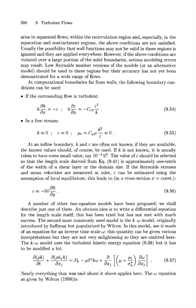
At computational boundaries far from walls, the following boundary conditions can be used:
If the surrounding
In a free stream:
flow is turbulent:
At an inflow boundary, lc and E are often not known; if they are available,
the known values should, of course, be used. If lc is not known, it is usually
taken t o have some small value, say
Ti2. The value of E should be selected
so that the length scale derived from Eq. (9.41) is approximately one-tenth
of the width of a shear layer or the domain size. If the Reynolds stresses
and mean velocities are measured at inlet, E can be estimated using the
assumption of local equilibrium; this leads to (in a cross-section x = const.):
A number of other two-equation models have been proposed; we shall
describe just one of them. An obvious idea is to write a differential equation
for the length scale itself; this has been tried but has not met with much
success. The second most commonly used model is the lc-w model, originally
introduced by Saffman but popularized by Wilcox. In this model, use is made
of an equation for an inverse time scale w; this quantity can be given various
interpretations but they are not very enlightening so they are omitted here.
The It-w model uses the turbulent kinetic energy equation (9.38) but it has
to be modified a bit:
Nearly everything that was said about it above applies here. The w equation
as given by Wilcox (1998)is:
9. Turbulent Flows
arise in separated flows; within the recirculation region and, especially, in the
separation and reattachment regions, the above conditions are not satisfied.
Usually the possibility that wall functions may not be valid in these regions is
ignored and they are applied everywhere. However, if the above conditions are
violated over a large portion of the solid boundaries, serious modeling errors
may result. Low Reynolds number versions of the models (or an alternative
model) should be used in these regions but their accuracy has not yet been
demonstrated for a wide range of flows.
At computational boundaries far from walls, the following boundary conditions can be used:
If the surrounding
In a free stream:
flow is turbulent:
At an inflow boundary, lc and E are often not known; if they are available,
the known values should, of course, be used. If lc is not known, it is usually
taken t o have some small value, say
Ti2. The value of E should be selected
so that the length scale derived from Eq. (9.41) is approximately one-tenth
of the width of a shear layer or the domain size. If the Reynolds stresses
and mean velocities are measured at inlet, E can be estimated using the
assumption of local equilibrium; this leads to (in a cross-section x = const.):
A number of other two-equation models have been proposed; we shall
describe just one of them. An obvious idea is to write a differential equation
for the length scale itself; this has been tried but has not met with much
success. The second most commonly used model is the lc-w model, originally
introduced by Saffman but popularized by Wilcox. In this model, use is made
of an equation for an inverse time scale w; this quantity can be given various
interpretations but they are not very enlightening so they are omitted here.
The It-w model uses the turbulent kinetic energy equation (9.38) but it has
to be modified a bit:
Nearly everything that was said about it above applies here. The w equation
as given by Wilcox (1998)is: