

9.2 Direct Numerical Simulation (DNS)
271
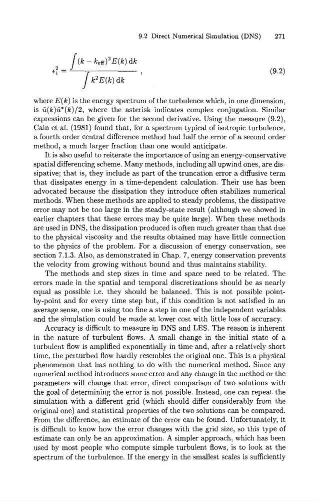
where E ( k ) is the energy spectrum of the turbulence which, in one dimension,
is C(k)C*(k)/2, where the asterisk indicates complex conjugation. Similar
expressions can be given for the second derivative. Using the measure (9.2),
Cain et al. (1981) found that, for a spectrum typical of isotropic turbulence,
a fourth order central difference method had half the error of a second order
method, a much larger fraction than one would anticipate.
It is also useful to reiterate the importance of using an energy-conservative
spatial differencing scheme. Many methods, including all upwind ones, are dissipative; that is, they include as part of the truncation error a diffusive term
that dissipates energy in a time-dependent calculation. Their use has been
advocated because the dissipation they introduce often stabilizes numerical
methods. When these methods are applied to steady problems, the dissipative
error may not be too large in the steady-state result (although we showed in
earlier chapters that these errors may be quite large). When these methods
are used in DNS, the dissipation produced is often much greater than that due
to the physical viscosity and the results obtained may have little connection
to the physics of the problem. For a discussion of energy conservation, see
section 7.1.3. Also, as demonstrated in Chap. 7, energy conservation prevents
the velocity from growing without bound and thus maintains stability.
The methods and step sizes in time and space need to be related. The
errors made in the spatial and temporal discretizations should be as nearly
equal as possible i.e. they should be balanced. This is not possible pointby-point and for every time step but, if this condition is not satisfied in an
average sense, one is using too fine a step in one of the independent variables
and the simulation could be made at lower cost with little loss of accuracy.
Accuracy is difficult to measure in DNS and LES. The reason is inherent
in the nature of turbulent flows. A small change in the initial state of a
turbulent flow is amplified exponentially in time and, after a relatively short
time, the perturbed flow hardly resembles the original one. This is a physical
phenomenon that has nothing to do with the numerical method. Since any
numerical method introduces some error and any change in the method or the
parameters will change that error, direct comparison of two solutions with
the goal of determining the error is not possible. Instead, one can repeat the
simulation with a different grid (which should differ considerably from the
original one) and statistical properties of the two solutions can be compared.
From the difference, an estimate of the error can be found. Unfortunately, it
is difficult to know how the error changes with the grid size, so this type of
estimate can only be an approximation. A simpler approach, which has been
used by most people who compute simple turbulent flows, is to look a t the
spectrum of the turbulence. If the energy in the smallest scales is sufficiently
271
where E ( k ) is the energy spectrum of the turbulence which, in one dimension,
is C(k)C*(k)/2, where the asterisk indicates complex conjugation. Similar
expressions can be given for the second derivative. Using the measure (9.2),
Cain et al. (1981) found that, for a spectrum typical of isotropic turbulence,
a fourth order central difference method had half the error of a second order
method, a much larger fraction than one would anticipate.
It is also useful to reiterate the importance of using an energy-conservative
spatial differencing scheme. Many methods, including all upwind ones, are dissipative; that is, they include as part of the truncation error a diffusive term
that dissipates energy in a time-dependent calculation. Their use has been
advocated because the dissipation they introduce often stabilizes numerical
methods. When these methods are applied to steady problems, the dissipative
error may not be too large in the steady-state result (although we showed in
earlier chapters that these errors may be quite large). When these methods
are used in DNS, the dissipation produced is often much greater than that due
to the physical viscosity and the results obtained may have little connection
to the physics of the problem. For a discussion of energy conservation, see
section 7.1.3. Also, as demonstrated in Chap. 7, energy conservation prevents
the velocity from growing without bound and thus maintains stability.
The methods and step sizes in time and space need to be related. The
errors made in the spatial and temporal discretizations should be as nearly
equal as possible i.e. they should be balanced. This is not possible pointby-point and for every time step but, if this condition is not satisfied in an
average sense, one is using too fine a step in one of the independent variables
and the simulation could be made at lower cost with little loss of accuracy.
Accuracy is difficult to measure in DNS and LES. The reason is inherent
in the nature of turbulent flows. A small change in the initial state of a
turbulent flow is amplified exponentially in time and, after a relatively short
time, the perturbed flow hardly resembles the original one. This is a physical
phenomenon that has nothing to do with the numerical method. Since any
numerical method introduces some error and any change in the method or the
parameters will change that error, direct comparison of two solutions with
the goal of determining the error is not possible. Instead, one can repeat the
simulation with a different grid (which should differ considerably from the
original one) and statistical properties of the two solutions can be compared.
From the difference, an estimate of the error can be found. Unfortunately, it
is difficult to know how the error changes with the grid size, so this type of
estimate can only be an approximation. A simpler approach, which has been
used by most people who compute simple turbulent flows, is to look a t the
spectrum of the turbulence. If the energy in the smallest scales is sufficiently