

8.11 Examples
263
has been enlarged to emphasize the differences between the solutions. The
expected second order convergence towards grid-independence can be seen.
A further increase in Reynolds number would make the pattern more and
more irregular, eventually the flow becomes turbulent.
Figure 8.20 shows instantaneous isobars and velocity vectors. The closed
pressure contours indicate the locations of vortex centers, where the pressure
has a local minimum.
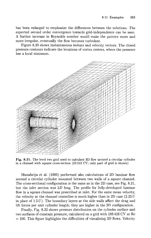
Fig. 8.21. The level two grid used to calculate 3D flow around a circular cylinder
in a channel with square cross-section (23 552 CV; only part of grid is shown)
Muzaferija et al. (1995) performed also calculations of 3D laminar flow
around a circular cylinder mounted between two walls of a square channel.
The cross-sectional configuration is the same as in the 2D case, see Fig. 8.21,
but the inlet section was 5D long. The profile for fully-developed laminar
flow in a square channel was prescribed at inlet. For the same mean velocity,
the velocity at the channel centerline is much higher than in 2D case (2.25 U
in place of 1.5 U). The boundary layers at the side walls affect the drag and
lift forces per unit cylinder length; they are higher in the 3D configuration.
Finally, Fig. 8.22 shows pressure distribution on the cylinder surface and
two surfaces of constant pressure, calculated on a grid with 188 416 CV at Re
= 100. This figure highlights the difficulties of visualizing 3D flows. Velocity
263
has been enlarged to emphasize the differences between the solutions. The
expected second order convergence towards grid-independence can be seen.
A further increase in Reynolds number would make the pattern more and
more irregular, eventually the flow becomes turbulent.
Figure 8.20 shows instantaneous isobars and velocity vectors. The closed
pressure contours indicate the locations of vortex centers, where the pressure
has a local minimum.
Fig. 8.21. The level two grid used to calculate 3D flow around a circular cylinder
in a channel with square cross-section (23 552 CV; only part of grid is shown)
Muzaferija et al. (1995) performed also calculations of 3D laminar flow
around a circular cylinder mounted between two walls of a square channel.
The cross-sectional configuration is the same as in the 2D case, see Fig. 8.21,
but the inlet section was 5D long. The profile for fully-developed laminar
flow in a square channel was prescribed at inlet. For the same mean velocity,
the velocity at the channel centerline is much higher than in 2D case (2.25 U
in place of 1.5 U). The boundary layers at the side walls affect the drag and
lift forces per unit cylinder length; they are higher in the 3D configuration.
Finally, Fig. 8.22 shows pressure distribution on the cylinder surface and
two surfaces of constant pressure, calculated on a grid with 188 416 CV at Re
= 100. This figure highlights the difficulties of visualizing 3D flows. Velocity