

8.8 Pressure-Correction Equation
251
The correction procedure can be continued, by introducing third, fourth
etc. corrections. The additional corrections tend to zero; it is rarely necessary
to go beyond the two already described as the pressure-correction equation
includes more severe approximations than the non-exact treatment of the
effects of grid non-orthogonality.
The inclusion of the second pressure correction has a minor effect on the
performance of the algorithm if the grid is nearly orthogonal. However, if the
angle between n and J is less than 45" in much of the domain, convergence
may be slow with only one correction. Strong under-relaxation (adding only
5-10% of pi to pm-l) and reduction of the under-relaxation factors for velocity
may help but a t a cost in efficiency. With two pressure-correction steps, the
performance found on orthogonal grids is obtained.
I
TWO corrections
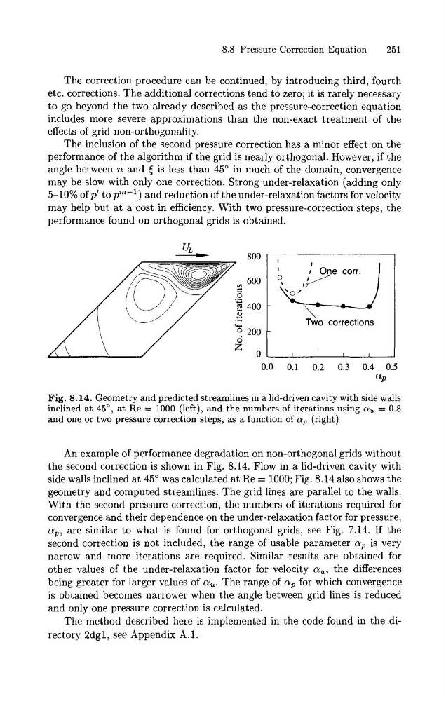
Fig. 8.14. Geometry and predicted streamlines in a lid-driven cavity with side walls
inclined at 4 5 O , at Re = 1000 (left), and the numbers of iterations using a, = 0.8
and one or two pressure correction steps, as a function of a, (right)
An example of performance degradation on non-orthogonal grids without
the second correction is shown in Fig. 8.14. Flow in a lid-driven cavity with
side walls inclined a t 45O was calculated a t Re = 1000; Fig. 8.14 also shows the
geometry and computed streamlines. The grid lines are parallel to the walls.
With the second pressure correction, the numbers of iterations required for
convergence and their dependence on the under-relaxation factor for pressure,
a,, are similar to what is found for orthogonal grids, see Fig. 7.14. If the
second correction is not included, the range of usable parameter a, is very
narrow and more iterations are required. Similar results are obtained for
other values of the under-relaxation factor for velocity a,, the differences
being greater for larger values of a,. The range of a, for which convergence
is obtained becomes narrower when the angle between grid lines is reduced
and only one pressure correction is calculated.
The method described here is implemented in the code found in the directory 2dg1, see Appendix A.1.
251
The correction procedure can be continued, by introducing third, fourth
etc. corrections. The additional corrections tend to zero; it is rarely necessary
to go beyond the two already described as the pressure-correction equation
includes more severe approximations than the non-exact treatment of the
effects of grid non-orthogonality.
The inclusion of the second pressure correction has a minor effect on the
performance of the algorithm if the grid is nearly orthogonal. However, if the
angle between n and J is less than 45" in much of the domain, convergence
may be slow with only one correction. Strong under-relaxation (adding only
5-10% of pi to pm-l) and reduction of the under-relaxation factors for velocity
may help but a t a cost in efficiency. With two pressure-correction steps, the
performance found on orthogonal grids is obtained.
I
TWO corrections
Fig. 8.14. Geometry and predicted streamlines in a lid-driven cavity with side walls
inclined at 4 5 O , at Re = 1000 (left), and the numbers of iterations using a, = 0.8
and one or two pressure correction steps, as a function of a, (right)
An example of performance degradation on non-orthogonal grids without
the second correction is shown in Fig. 8.14. Flow in a lid-driven cavity with
side walls inclined a t 45O was calculated a t Re = 1000; Fig. 8.14 also shows the
geometry and computed streamlines. The grid lines are parallel to the walls.
With the second pressure correction, the numbers of iterations required for
convergence and their dependence on the under-relaxation factor for pressure,
a,, are similar to what is found for orthogonal grids, see Fig. 7.14. If the
second correction is not included, the range of usable parameter a, is very
narrow and more iterations are required. Similar results are obtained for
other values of the under-relaxation factor for velocity a,, the differences
being greater for larger values of a,. The range of a, for which convergence
is obtained becomes narrower when the angle between grid lines is reduced
and only one pressure correction is calculated.
The method described here is implemented in the code found in the directory 2dg1, see Appendix A.1.