

222
8. Complex Geometries
volume types. In principle, any type of method (FD, FV, FE) can be adapted
to this kind of grid.
Another approach to automatic grid generation is to cover the solution
domain with a (coarse) Cartesian grid, and adjust the cells cut by domain
boundaries to fit the boundary. The problem with this approach is that the
cells near boundary are irregular and may require special treatment. However,
if this is done on a very coarse level and the grid is then refined several times,
the irregularity is limited to a few locations and will not affect the accuracy
much but the degree of boundary irregularity is limited.
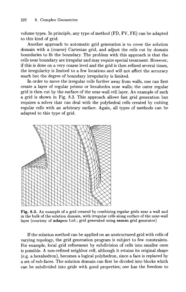
In order to move the irregular cells further away from walls, one can first
create a layer of regular prisms or hexahedra near walls; the outer regular
grid is then cut by the surface of the near-wall cell layer. An example of such
a grid is shown in Fig. 8.3. This approach allows fast grid generation but
requires a solver that can deal with the polyhedral cells created by cutting
regular cells with an arbitrary surface. Again, all types of methods can be
adapted to this type of grid.
Fig. 8.3. An example of a grid created by combining regular grids near a wall and
in the bulk of the solution domain, with irregular cells along surface of the near-wall
layer (courtesy of adapco Ltd.; grid generated using samm grid generator)
If the solution method can be applied on an unstructured grid with cells of
varying topology, the grid generation program is subject to few constraints.
For example, local grid refinement by subdivision of cells into smaller ones
is possible. A non-refined neighbor cell, although it retains its original shape
(e.g. a hexahedron), becomes a logical polyhedron, since a face is replaced by
a set of sub-faces. The solution domain can first be divided into blocks which
can be subdivided into grids with good properties; one has the freedom to
8. Complex Geometries
volume types. In principle, any type of method (FD, FV, FE) can be adapted
to this kind of grid.
Another approach to automatic grid generation is to cover the solution
domain with a (coarse) Cartesian grid, and adjust the cells cut by domain
boundaries to fit the boundary. The problem with this approach is that the
cells near boundary are irregular and may require special treatment. However,
if this is done on a very coarse level and the grid is then refined several times,
the irregularity is limited to a few locations and will not affect the accuracy
much but the degree of boundary irregularity is limited.
In order to move the irregular cells further away from walls, one can first
create a layer of regular prisms or hexahedra near walls; the outer regular
grid is then cut by the surface of the near-wall cell layer. An example of such
a grid is shown in Fig. 8.3. This approach allows fast grid generation but
requires a solver that can deal with the polyhedral cells created by cutting
regular cells with an arbitrary surface. Again, all types of methods can be
adapted to this type of grid.
Fig. 8.3. An example of a grid created by combining regular grids near a wall and
in the bulk of the solution domain, with irregular cells along surface of the near-wall
layer (courtesy of adapco Ltd.; grid generated using samm grid generator)
If the solution method can be applied on an unstructured grid with cells of
varying topology, the grid generation program is subject to few constraints.
For example, local grid refinement by subdivision of cells into smaller ones
is possible. A non-refined neighbor cell, although it retains its original shape
(e.g. a hexahedron), becomes a logical polyhedron, since a face is replaced by
a set of sub-faces. The solution domain can first be divided into blocks which
can be subdivided into grids with good properties; one has the freedom to