

198
7. Solution of the Navier-Stokes Equations
We again denote the right hand side as QF; however, this quantity is not the
one obtained previously. Inserting the central difference approximations for
pressure derivatives, we find:
The system of algebraic equations for the pressure has the form:
where the coefficients are:
This equation has the same form as Eq. (7.117) but it involves nodes which
are 2Ax apart! It is a discretized Poisson equation on a grid twice as coarse
as the basic one but the equations split into four unconnected systems, one
with i and j both even, one with i even and j odd, one with i odd and j even,
and one with both odd. Each of these systems gives a different solution. For
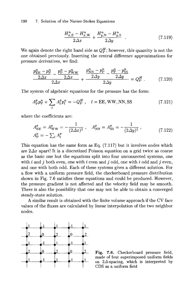
a flow with a uniform pressure field, the checkerboard pressure distribution
shown in Fig. 7.6 satisfies these equations and could be produced. However,
the pressure gradient is not affected and the velocity field may be smooth.
There is also the possibility that one may not be able to obtain a converged
steady-state solution.
A similar result is obtained with the finite volume approach if the CV face
values of the fluxes are calculated by linear interpolation of the two neighbor
nodes.
. . 2
. . O
.
.
2
. . O
..- 1
j2
Fig. 7.6. Checkerboard pressure field,
made of four superimposed uniform fields
1' on 2d-spacing, which is interpreted by
CDS as a uniform field
7. Solution of the Navier-Stokes Equations
We again denote the right hand side as QF; however, this quantity is not the
one obtained previously. Inserting the central difference approximations for
pressure derivatives, we find:
The system of algebraic equations for the pressure has the form:
where the coefficients are:
This equation has the same form as Eq. (7.117) but it involves nodes which
are 2Ax apart! It is a discretized Poisson equation on a grid twice as coarse
as the basic one but the equations split into four unconnected systems, one
with i and j both even, one with i even and j odd, one with i odd and j even,
and one with both odd. Each of these systems gives a different solution. For
a flow with a uniform pressure field, the checkerboard pressure distribution
shown in Fig. 7.6 satisfies these equations and could be produced. However,
the pressure gradient is not affected and the velocity field may be smooth.
There is also the possibility that one may not be able to obtain a converged
steady-state solution.
A similar result is obtained with the finite volume approach if the CV face
values of the fluxes are calculated by linear interpolation of the two neighbor
nodes.
. . 2
. . O
.
.
2
. . O
..- 1
j2
Fig. 7.6. Checkerboard pressure field,
made of four superimposed uniform fields
1' on 2d-spacing, which is interpreted by
CDS as a uniform field