

7.4 Other Methods
179
method; in this step, the pressure is treated explicitly. Why use it at all? The
fractional step method of Kim and Moin (1985) provides an approach that
does not use pressure in the predictor step. It is also important to recall that
the role of the pressure in an incompressible flow is to enforce continuity; in
some sense, it is more a mathematical variable than a physical one.
The fractional step concept is more a generic approach than a particular
method. It is based on ideas similar to those that led to the alternating direction implicit method in Chap. 5 . It is essentially an approximate factorization
of a method; the underlying method need not be implicit. To see how this
might work, we take the simplest case, the Euler explicit advancement of the
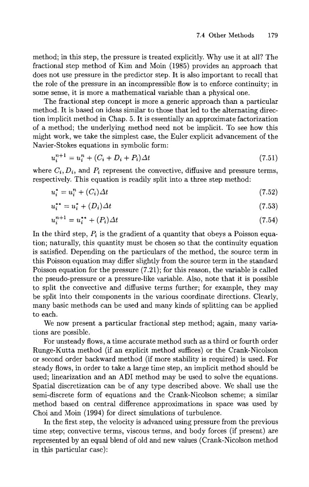
Navier-Stokes equations in symbolic form:
U;+'
= U: + (Ci + Di + Pi)&
(7.51)
where Ci, Di, and Pi represent the convective, diffusive and pressure terms,
respectively. This equation is readily split into a three step method:
ut = ul + (Ci)At
(7.52)
In the third step, Pi is the gradient of a quantity that obeys a Poisson equation; naturally, this quantity must be chosen so that the continuity equation
is satisfied. Depending on the particulars of the method, the source term in
this Poisson equation may differ slightly from the source term in the standard
Poisson equation for the pressure (7.21); for this reason, the variable is called
the pseudo-pressure or a pressure-like variable. Also, note that it is possible
to split the convective and diffusive terms further; for example, they may
be split into their components in the various coordinate directions. Clearly,
many basic methods can be used and many kinds of splitting can be applied
to each.
We now present a particular fractional step method; again, many variations are possible.
For unsteady flows, a time accurate method such as a third or fourth order
Runge-Kutta method (if an explicit method suffices) or the Crank-Nicolson
or second order backward method (if more stability is required) is used. For
steady flows, in order to take a large time step, an implicit method should be
used; linearization and an AD1 method may be used to solve the equations.
Spatial discretization can be of any type described above. We shall use the
semi-discrete form of equations and the Crank-Nicolson scheme; a similar
method based on central difference approximations in space was used by
Choi and Moin (1994) for direct simulations of turbulence.
In the first step, the velocity is advanced using pressure from the previous
time step; convective terms, viscous terms, and body forces (if present) are
represented by an equal blend of old and new values (Crank-Nicolson method
in this particular case):
179
method; in this step, the pressure is treated explicitly. Why use it at all? The
fractional step method of Kim and Moin (1985) provides an approach that
does not use pressure in the predictor step. It is also important to recall that
the role of the pressure in an incompressible flow is to enforce continuity; in
some sense, it is more a mathematical variable than a physical one.
The fractional step concept is more a generic approach than a particular
method. It is based on ideas similar to those that led to the alternating direction implicit method in Chap. 5 . It is essentially an approximate factorization
of a method; the underlying method need not be implicit. To see how this
might work, we take the simplest case, the Euler explicit advancement of the
Navier-Stokes equations in symbolic form:
U;+'
= U: + (Ci + Di + Pi)&
(7.51)
where Ci, Di, and Pi represent the convective, diffusive and pressure terms,
respectively. This equation is readily split into a three step method:
ut = ul + (Ci)At
(7.52)
In the third step, Pi is the gradient of a quantity that obeys a Poisson equation; naturally, this quantity must be chosen so that the continuity equation
is satisfied. Depending on the particulars of the method, the source term in
this Poisson equation may differ slightly from the source term in the standard
Poisson equation for the pressure (7.21); for this reason, the variable is called
the pseudo-pressure or a pressure-like variable. Also, note that it is possible
to split the convective and diffusive terms further; for example, they may
be split into their components in the various coordinate directions. Clearly,
many basic methods can be used and many kinds of splitting can be applied
to each.
We now present a particular fractional step method; again, many variations are possible.
For unsteady flows, a time accurate method such as a third or fourth order
Runge-Kutta method (if an explicit method suffices) or the Crank-Nicolson
or second order backward method (if more stability is required) is used. For
steady flows, in order to take a large time step, an implicit method should be
used; linearization and an AD1 method may be used to solve the equations.
Spatial discretization can be of any type described above. We shall use the
semi-discrete form of equations and the Crank-Nicolson scheme; a similar
method based on central difference approximations in space was used by
Choi and Moin (1994) for direct simulations of turbulence.
In the first step, the velocity is advanced using pressure from the previous
time step; convective terms, viscous terms, and body forces (if present) are
represented by an equal blend of old and new values (Crank-Nicolson method
in this particular case):