

152
6. Methods for Unsteady Problems
6.4 Examples
In order to demonstrate the performance of some of the methods described
above, we look first at the unsteady version of the example problem of Chap.
3. The problem to be solved is given by Eq. (6.23), with the following initial
and boundary conditions: at t = 0, &, = 0; for all subsequent times, 4 = 0
at x = 0, q5= 1 at x = L = 1, p = 1, u = 1 and r = 0 . 1 . Since the boundary
conditions do not change in time, the solution develops from the initial zero
field to the steady state solution given in Sect. 3.11. For spatial discretization,
second order CDS is used. For temporal discretization, we use both explicit
and implicit first order Euler methods, the Crank-Nicolson method and the
fully implicit method with three time levels.
We first demonstrate what happens when the explicit Euler scheme (which
is only conditionally stable) is used with time steps which violate the stability
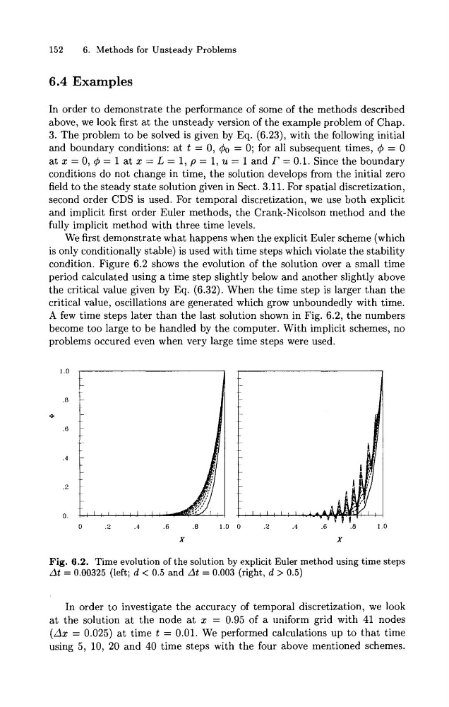
condition. Figure 6.2 shows the evolution of the solution over a small time
period calculated using a time step slightly below and another slightly above
the critical value given by Eq. (6.32). When the time step is larger than the
critical value, oscillations are generated which grow unboundedly with time.
A few time steps later than the last solution shown in Fig. 6.2, the numbers
become too large to be handled by the computer. With implicit schemes, no
problems occured even when very large time steps were used.
Fig. 6.2. Time evolution of the solution by explicit Euler method using time steps
At = 0.00325 (left; d < 0.5 and At = 0.003 (right, d > 0.5)
In order to investigate the accuracy of temporal discretization, we look
at the solution at the node a t x = 0.95 of a uniform grid with 41 nodes
(Ax = 0.025) a t time t = 0.01. We performed calculations up to that time
using 5, 10, 20 and 40 time steps with the four above mentioned schemes.
6. Methods for Unsteady Problems
6.4 Examples
In order to demonstrate the performance of some of the methods described
above, we look first at the unsteady version of the example problem of Chap.
3. The problem to be solved is given by Eq. (6.23), with the following initial
and boundary conditions: at t = 0, &, = 0; for all subsequent times, 4 = 0
at x = 0, q5= 1 at x = L = 1, p = 1, u = 1 and r = 0 . 1 . Since the boundary
conditions do not change in time, the solution develops from the initial zero
field to the steady state solution given in Sect. 3.11. For spatial discretization,
second order CDS is used. For temporal discretization, we use both explicit
and implicit first order Euler methods, the Crank-Nicolson method and the
fully implicit method with three time levels.
We first demonstrate what happens when the explicit Euler scheme (which
is only conditionally stable) is used with time steps which violate the stability
condition. Figure 6.2 shows the evolution of the solution over a small time
period calculated using a time step slightly below and another slightly above
the critical value given by Eq. (6.32). When the time step is larger than the
critical value, oscillations are generated which grow unboundedly with time.
A few time steps later than the last solution shown in Fig. 6.2, the numbers
become too large to be handled by the computer. With implicit schemes, no
problems occured even when very large time steps were used.
Fig. 6.2. Time evolution of the solution by explicit Euler method using time steps
At = 0.00325 (left; d < 0.5 and At = 0.003 (right, d > 0.5)
In order to investigate the accuracy of temporal discretization, we look
at the solution at the node a t x = 0.95 of a uniform grid with 41 nodes
(Ax = 0.025) a t time t = 0.01. We performed calculations up to that time
using 5, 10, 20 and 40 time steps with the four above mentioned schemes.