

Appendix C Useful Theoretical Approaches and Formulas
491
C.4 Summary of Basic Irrotational Flow Properties
In Sect. C.3 it was shown that the conditions of irrotationality impose an
existence of the velocity potential function ¢, such that velocity components
u(x, y, z, t), v(x, y, z, t) and w(x, y, z, t) are the derivatives of function ¢ with
respect to x, y and z, correspondingly. The velocity potential function may be
used for any kind of irrotational flow, steady or unsteady, and two- or threedimensional. It is also used in the study of turbulent flow, provided the velocity
potential, ¢, refers to the time-average motion. Note that the dimension of the
velocity potential function is [m 2 s- 1 ].
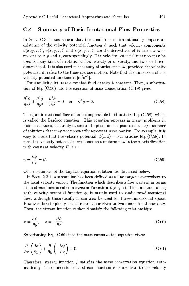
For simplicity, let us assume that fluid density is constant. Then, a substitution of Eq. (C.36) into the equation of mass conservation (C.19) gives:
(C.58)
Thus, an irrotational flow of an incompressible fluid satisfies Eq. (C.58), which
is called the Laplace equation. This equation appears in many problems in
fluid mechanics, electrodynamics and optics, and it possesses a large number
of solutions that may not necessarily represent wave motion. For example, it is
easy to check that the velocity potential, ¢(x, z) = U x, satisfies Eq. (C.58). In
fact, this velocity potential corresponds to a uniform flow in the x-axis direction
with constant velocity, U, i. e.:
o¢
u= -
= U.
ox
Other examples of the Laplace equation solution are discussed below.
(C.59)
In Sect. 2.3.1, a streamline has been defined as a line tangent everywhere to
the local velocity vector. The function which describes a flow pattern in terms
of its streamlines is called a stream function 1/J (x, y, z). This function, along
with velocity potential function ¢, is mainly used to study two-dimensional
flow, although theoretically it can also be used for three-dimensional space.
However, for simplicity, let us restrict ourselves to two-dimensional flow only.
Then, the stream function 1/J should satisfy the following relationships:
o1/J
u = -
o '
y
o1/J
V = - - .
ox
Substituting Eq. (C.60) into the mass conservation equation gives:
~ (o1/J) + ~ (_ o1/J) == O.
ox oy
oy
ox
(C.60)
(C.61)
Therefore, stream function 1/J satisfies the mass conservation equation automatically. The dimension of a stream function 1/J is identical to the velocity
491
C.4 Summary of Basic Irrotational Flow Properties
In Sect. C.3 it was shown that the conditions of irrotationality impose an
existence of the velocity potential function ¢, such that velocity components
u(x, y, z, t), v(x, y, z, t) and w(x, y, z, t) are the derivatives of function ¢ with
respect to x, y and z, correspondingly. The velocity potential function may be
used for any kind of irrotational flow, steady or unsteady, and two- or threedimensional. It is also used in the study of turbulent flow, provided the velocity
potential, ¢, refers to the time-average motion. Note that the dimension of the
velocity potential function is [m 2 s- 1 ].
For simplicity, let us assume that fluid density is constant. Then, a substitution of Eq. (C.36) into the equation of mass conservation (C.19) gives:
(C.58)
Thus, an irrotational flow of an incompressible fluid satisfies Eq. (C.58), which
is called the Laplace equation. This equation appears in many problems in
fluid mechanics, electrodynamics and optics, and it possesses a large number
of solutions that may not necessarily represent wave motion. For example, it is
easy to check that the velocity potential, ¢(x, z) = U x, satisfies Eq. (C.58). In
fact, this velocity potential corresponds to a uniform flow in the x-axis direction
with constant velocity, U, i. e.:
o¢
u= -
= U.
ox
Other examples of the Laplace equation solution are discussed below.
(C.59)
In Sect. 2.3.1, a streamline has been defined as a line tangent everywhere to
the local velocity vector. The function which describes a flow pattern in terms
of its streamlines is called a stream function 1/J (x, y, z). This function, along
with velocity potential function ¢, is mainly used to study two-dimensional
flow, although theoretically it can also be used for three-dimensional space.
However, for simplicity, let us restrict ourselves to two-dimensional flow only.
Then, the stream function 1/J should satisfy the following relationships:
o1/J
u = -
o '
y
o1/J
V = - - .
ox
Substituting Eq. (C.60) into the mass conservation equation gives:
~ (o1/J) + ~ (_ o1/J) == O.
ox oy
oy
ox
(C.60)
(C.61)
Therefore, stream function 1/J satisfies the mass conservation equation automatically. The dimension of a stream function 1/J is identical to the velocity