

332
9 Experimental Methods in Fluid Mechanics
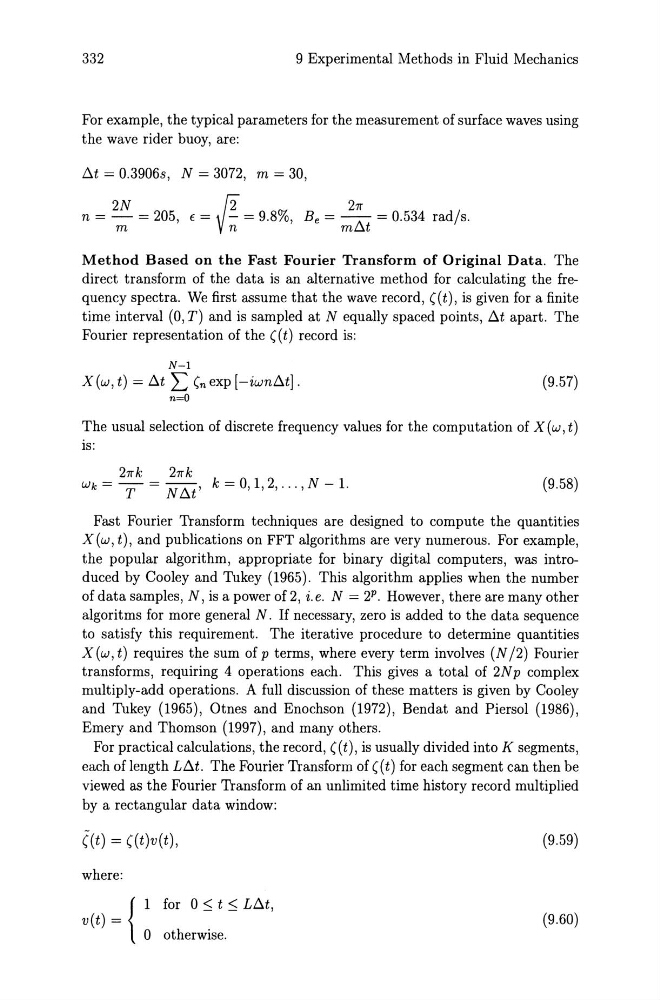
For example, the typical parameters for the measurement of surface waves using
the wave rider buoy, are:
.6.t = 0.39068, N = 3072, m = 30,
2N
~
27r
n = - = 205, f = - = 9.8%, Be = ----;\ = 0.534 rad/s.
m
n
mLl.t
Method Based on the Fast Fourier Transform of Original Data. The
direct transform of the data is an alternative method for calculating the frequency spectra. We first assume that the wave record, ((t), is given for a finite
time interval (0, T) and is sampled at N equally spaced points, .6.t apart. The
Fourier representation of the (( t) record is:
N-l
X(w, t) =.6.t L (nexp [-iwn.6.t].
(9.57)
n=O
The usual selection of discrete frequency values for the computation of X (w, t)
is:
27rk
27rk
Wk = T = N .6.t' k = 0,1,2, ... , N - 1.
(9.58)
Fast Fourier Transform techniques are designed to compute the quantities
X (w, t), and publications on FFT algorithms are very numerous. For example,
the popular algorithm, appropriate for binary digital computers, was introduced by Cooley and Thkey (1965). This algorithm applies when the number
of data samples, N, is a power of 2, i. e. N = 2 P . However, there are many other
algoritms for more general N. If necessary, zero is added to the data sequence
to satisfy this requirement. The iterative procedure to determine quantities
X(w, t) requires the sum of p terms, where every term involves (N /2) Fourier
transforms, requiring 4 operations each. This gives a total of 2N p complex
multiply-add operations. A full discussion of these matters is given by Cooley
and Thkey (1965), Otnes and Enochson (1972), Bendat and Piersol (1986),
Emery and Thomson (1997), and many others.
For practical calculations, the record, ((t), is usually divided into K segments,
each of length L.6.t. The Fourier Transform of ((t) for each segment can then be
viewed as the Fourier Transform of an unlimited time history record multiplied
by a rectangular data window:
((t) = ((t)v(t),
where:
{
I for 0:::; t :::; L.6.t,
v(t) = o otherwise.
(9.59)
(9.60)
9 Experimental Methods in Fluid Mechanics
For example, the typical parameters for the measurement of surface waves using
the wave rider buoy, are:
.6.t = 0.39068, N = 3072, m = 30,
2N
~
27r
n = - = 205, f = - = 9.8%, Be = ----;\ = 0.534 rad/s.
m
n
mLl.t
Method Based on the Fast Fourier Transform of Original Data. The
direct transform of the data is an alternative method for calculating the frequency spectra. We first assume that the wave record, ((t), is given for a finite
time interval (0, T) and is sampled at N equally spaced points, .6.t apart. The
Fourier representation of the (( t) record is:
N-l
X(w, t) =.6.t L (nexp [-iwn.6.t].
(9.57)
n=O
The usual selection of discrete frequency values for the computation of X (w, t)
is:
27rk
27rk
Wk = T = N .6.t' k = 0,1,2, ... , N - 1.
(9.58)
Fast Fourier Transform techniques are designed to compute the quantities
X (w, t), and publications on FFT algorithms are very numerous. For example,
the popular algorithm, appropriate for binary digital computers, was introduced by Cooley and Thkey (1965). This algorithm applies when the number
of data samples, N, is a power of 2, i. e. N = 2 P . However, there are many other
algoritms for more general N. If necessary, zero is added to the data sequence
to satisfy this requirement. The iterative procedure to determine quantities
X(w, t) requires the sum of p terms, where every term involves (N /2) Fourier
transforms, requiring 4 operations each. This gives a total of 2N p complex
multiply-add operations. A full discussion of these matters is given by Cooley
and Thkey (1965), Otnes and Enochson (1972), Bendat and Piersol (1986),
Emery and Thomson (1997), and many others.
For practical calculations, the record, ((t), is usually divided into K segments,
each of length L.6.t. The Fourier Transform of ((t) for each segment can then be
viewed as the Fourier Transform of an unlimited time history record multiplied
by a rectangular data window:
((t) = ((t)v(t),
where:
{
I for 0:::; t :::; L.6.t,
v(t) = o otherwise.
(9.59)
(9.60)