

9.5 Spectral and Statistical Analysis of Time Series
331
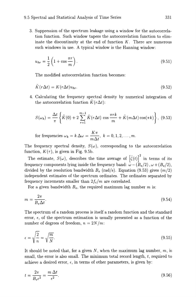
3. Suppression of the spectrum leakage using a window for the autocorrelation function. Such window tapers the autocorrelation function to eliminate the discontinuity at the end of function K. There are numerous
such windows in use. A typical window is the Hanning window:
1 (
7fT)
Uhr = ' 2 1 + cos m .
(9.51 )
The modified autocorrelation function becomes:
K(rt:.t) = K(rt:.t)Uhr.
(9.52)
4. Calculating the frequency spectral density by numerical integration of
the autocorrelation function K (r t:.t):
t:.t { _
m-l _
7rrk
_
}
S(Wk) = -;- K(O) + 2 ?; K(rt:.t) cos --:;;;- + K(mt:.t) cos(Jrk) , (9.53)
K7r
for frequencies Wk = k t:.w = mt:.t' k = 0, 1,2, ... , m.
The frequency spectral density, S(w), corresponding to the autocorrelation
function, K(T), is given in Fig. 9.5b.
The estimate, S(w), describes the time average of [C(t)f in terms of its
frequency components lying inside the frequency band: w - (Be /2), w + (Be /2),
divided by the resolution bandwidth Be (rad/s). Equation (9.53) gives (m/2)
independent estimates of the spectrum ordinates. The ordinates separated by
frequency increments smaller than 2fc/m are correlated.
For a given bandwidth Be, the required maximum lag number m is:
(9.54)
The spectrum of a random process is itself a random function and the standard
error, E, of the spectrum estimation is usually presented as a function of the
number of degrees of freedom, n = 2N /m:
(9.55)
It should be noted that, for a given N, when the maximum lag number, m, is
small, the error is also small. The minimum total record length, t, required to
achieve a desired error, E, in terms of other parameters, is given by:
(9.56)
331
3. Suppression of the spectrum leakage using a window for the autocorrelation function. Such window tapers the autocorrelation function to eliminate the discontinuity at the end of function K. There are numerous
such windows in use. A typical window is the Hanning window:
1 (
7fT)
Uhr = ' 2 1 + cos m .
(9.51 )
The modified autocorrelation function becomes:
K(rt:.t) = K(rt:.t)Uhr.
(9.52)
4. Calculating the frequency spectral density by numerical integration of
the autocorrelation function K (r t:.t):
t:.t { _
m-l _
7rrk
_
}
S(Wk) = -;- K(O) + 2 ?; K(rt:.t) cos --:;;;- + K(mt:.t) cos(Jrk) , (9.53)
K7r
for frequencies Wk = k t:.w = mt:.t' k = 0, 1,2, ... , m.
The frequency spectral density, S(w), corresponding to the autocorrelation
function, K(T), is given in Fig. 9.5b.
The estimate, S(w), describes the time average of [C(t)f in terms of its
frequency components lying inside the frequency band: w - (Be /2), w + (Be /2),
divided by the resolution bandwidth Be (rad/s). Equation (9.53) gives (m/2)
independent estimates of the spectrum ordinates. The ordinates separated by
frequency increments smaller than 2fc/m are correlated.
For a given bandwidth Be, the required maximum lag number m is:
(9.54)
The spectrum of a random process is itself a random function and the standard
error, E, of the spectrum estimation is usually presented as a function of the
number of degrees of freedom, n = 2N /m:
(9.55)
It should be noted that, for a given N, when the maximum lag number, m, is
small, the error is also small. The minimum total record length, t, required to
achieve a desired error, E, in terms of other parameters, is given by:
(9.56)