

9.5 Spectral and Statistical Analysis of Time Series
r
\ I
o
2
I \
I
3
I \
\
4
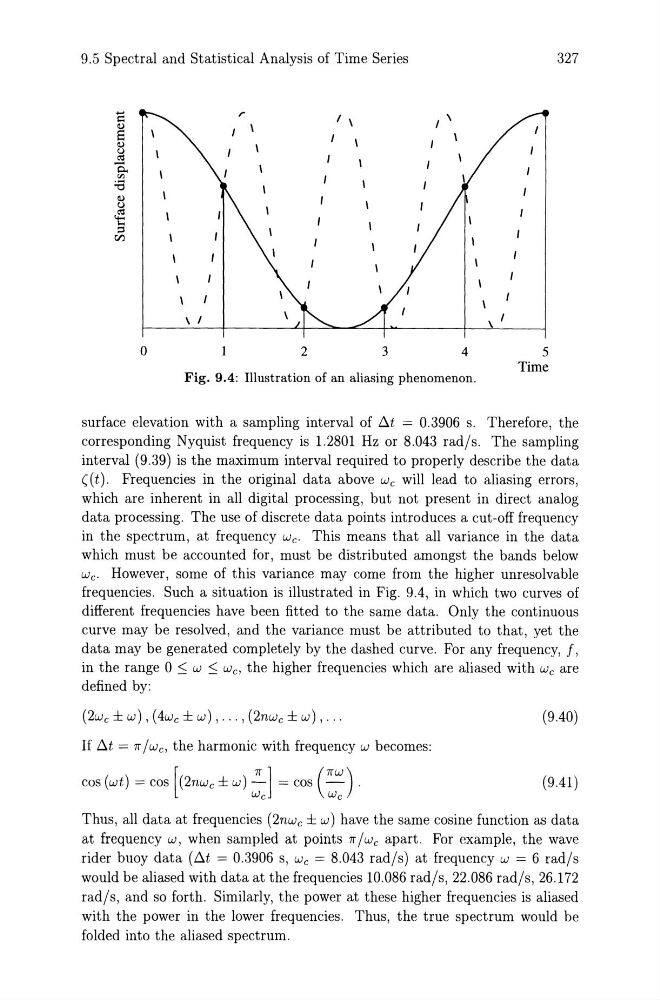
Fig. 9.4: Illustration of an aliasing phenomenon.
\ I
5
Time
327
surface elevation with a sampling interval of t1t = 0.3906 s. Therefore, the
corresponding Nyquist frequency is 1.2801 Hz or 8.043 rad/s. The sampling
interval (9.39) is the maximum interval required to properly describe the data
((t). Frequencies in the original data above We will lead to aliasing errors,
which are inherent in all digital processing, but not present in direct analog
data processing. The use of discrete data points introduces a cut-off frequency
in the spectrum, at frequency We' This means that all variance in the data
which must be accounted for, must be distributed amongst the bands below
We' However, some of this variance may come from the higher unresolvable
frequencies. Such a situation is illustrated in Fig. 9.4, in which two curves of
different frequencies have been fitted to the same data. Only the continuous
curve may be resolved, and the variance must be attributed to that, yet the
data may be generated completely by the dashed curve. For any frequency, f,
in the range 0 :::; W :::; We, the higher frequencies which are aliased with We are
defined by:
(2we ± w) , (4wc ± w) , ... , (2nwe ± w) , ...
(9.40)
If t1t = n-jwc, the harmonic with frequency W becomes:
cos (wt) = cos [( 2nwc ± w) ~J = cos (::) .
(9.41)
Thus, all data at frequencies (2nwc ± w) have the same cosine function as data
at frequency w, when sampled at points IT/we apart. For example, the wave
rider buoy data (t1t = 0.3906 s, We = 8.043 rad/s) at frequency w = 6 rad/s
would be aliased with data at the frequencies 10.086 rad/s, 22.086 rad/s, 26.172
rad/s, and so forth. Similarly, the power at these higher frequencies is aliased
with the power in the lower frequencies. Thus, the true spectrum would be
folded into the aliased spectrum.
r
\ I
o
2
I \
I
3
I \
\
4
Fig. 9.4: Illustration of an aliasing phenomenon.
\ I
5
Time
327
surface elevation with a sampling interval of t1t = 0.3906 s. Therefore, the
corresponding Nyquist frequency is 1.2801 Hz or 8.043 rad/s. The sampling
interval (9.39) is the maximum interval required to properly describe the data
((t). Frequencies in the original data above We will lead to aliasing errors,
which are inherent in all digital processing, but not present in direct analog
data processing. The use of discrete data points introduces a cut-off frequency
in the spectrum, at frequency We' This means that all variance in the data
which must be accounted for, must be distributed amongst the bands below
We' However, some of this variance may come from the higher unresolvable
frequencies. Such a situation is illustrated in Fig. 9.4, in which two curves of
different frequencies have been fitted to the same data. Only the continuous
curve may be resolved, and the variance must be attributed to that, yet the
data may be generated completely by the dashed curve. For any frequency, f,
in the range 0 :::; W :::; We, the higher frequencies which are aliased with We are
defined by:
(2we ± w) , (4wc ± w) , ... , (2nwe ± w) , ...
(9.40)
If t1t = n-jwc, the harmonic with frequency W becomes:
cos (wt) = cos [( 2nwc ± w) ~J = cos (::) .
(9.41)
Thus, all data at frequencies (2nwc ± w) have the same cosine function as data
at frequency w, when sampled at points IT/we apart. For example, the wave
rider buoy data (t1t = 0.3906 s, We = 8.043 rad/s) at frequency w = 6 rad/s
would be aliased with data at the frequencies 10.086 rad/s, 22.086 rad/s, 26.172
rad/s, and so forth. Similarly, the power at these higher frequencies is aliased
with the power in the lower frequencies. Thus, the true spectrum would be
folded into the aliased spectrum.