

326
9 Experimental Methods in Fluid Mechanics
on the model have to be multiplied by 10 to obtain expected velocities in the
prototype.
Equations (9.31) and (9.35) yield the following relationship for time scaling
under the Froude criterion as:
(9.36)
Other similitude criteria and approaches to model similitude are discussed in
more detail by Le Mehaute (1990) and Hughes (1993).
9.5 Spectral and Statistical Analysis of Time Series
Most experimental data on flows in the ocean are time series of surface elevation, velocities, pressure and other parameters for a given point or for a
given profile (for example ADCP records). Except maybe tides, these data represent random oscillations and special statistical and spectral methods have
to be used to analyze data. A very comprehensive overview of the analytical
and numerical methods of data processing is given by Emery and Thomson
(1997). Therefore, in this section we briefly summarize the practical methods
for evaluation of experimental frequency spectra and statistics.
9.5.1 Data Sampling
Let us assume that a record is of duration t. The digital data consists of N
data values with an equally-spaced sampling ilt. Thus:
(n=((to+nilt) n=I,2, ... ,N,
(9.37)
where to is an arbitrary initial time. During the experimental planning stage,
particular care should be taken in the adoption of the ilt value. Let us assume
that the frequency band of interest ranges from 0 to fe Hz (we = 27rfe rad/s).
The number, N, of discrete samples, required to describe (( t), should satisfy
the following relationship:
t
wet
N = - - = 2fet = -
1/2fe
7r '
or:
t
1
7r
ilt = - = - = -.
N
2fe We
(9.38)
(9.39)
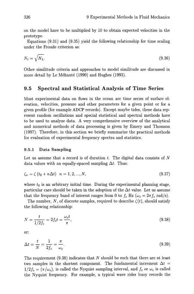
The requirement (9.38) indicates that N should be such that there are at least
two samples in the shortest component. The fundamental increment ilt =
1/2fe = (7r/we), is called the Nyquist sampling interval, and Ie or We is called
the Nyquist frequency. For example, a typical wave rider buoy records the
9 Experimental Methods in Fluid Mechanics
on the model have to be multiplied by 10 to obtain expected velocities in the
prototype.
Equations (9.31) and (9.35) yield the following relationship for time scaling
under the Froude criterion as:
(9.36)
Other similitude criteria and approaches to model similitude are discussed in
more detail by Le Mehaute (1990) and Hughes (1993).
9.5 Spectral and Statistical Analysis of Time Series
Most experimental data on flows in the ocean are time series of surface elevation, velocities, pressure and other parameters for a given point or for a
given profile (for example ADCP records). Except maybe tides, these data represent random oscillations and special statistical and spectral methods have
to be used to analyze data. A very comprehensive overview of the analytical
and numerical methods of data processing is given by Emery and Thomson
(1997). Therefore, in this section we briefly summarize the practical methods
for evaluation of experimental frequency spectra and statistics.
9.5.1 Data Sampling
Let us assume that a record is of duration t. The digital data consists of N
data values with an equally-spaced sampling ilt. Thus:
(n=((to+nilt) n=I,2, ... ,N,
(9.37)
where to is an arbitrary initial time. During the experimental planning stage,
particular care should be taken in the adoption of the ilt value. Let us assume
that the frequency band of interest ranges from 0 to fe Hz (we = 27rfe rad/s).
The number, N, of discrete samples, required to describe (( t), should satisfy
the following relationship:
t
wet
N = - - = 2fet = -
1/2fe
7r '
or:
t
1
7r
ilt = - = - = -.
N
2fe We
(9.38)
(9.39)
The requirement (9.38) indicates that N should be such that there are at least
two samples in the shortest component. The fundamental increment ilt =
1/2fe = (7r/we), is called the Nyquist sampling interval, and Ie or We is called
the Nyquist frequency. For example, a typical wave rider buoy records the