

S.5 Diffusion and Mixing in Estuaries
293
and at the bottom (z = - h), velocity u vanishes:
u = 0, at z = -h.
(S.104)
The solution on Eq. (S.102) with boundary conditions (S.103) and (S.104) takes
the form (Officer, 1976):
u(z) = -- 1 - -
+ - - - 1 - 9 - - S -
,
3Q [
(Z)2] 1 g)"h 3 [ (Z)2 (Z)3]
2 h
h
4S PwAz
h
h
(S.105)
in which Q is the total discharge per unit width. In particular, the velocity at
the surface is given by:
3Q
1 g)"h 3
u(O) = 2h + 4S PwAz'
(S.106)
and the mean velocity becomes:
- Q
u= -.
h
(S.107)
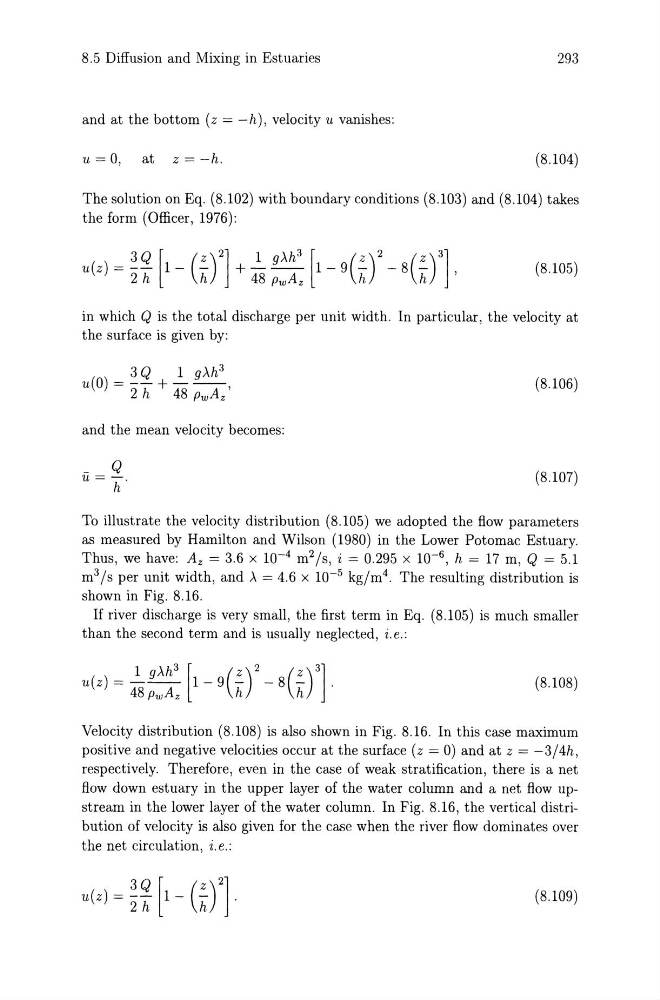
To illustrate the velocity distribution (S.105) we adopted the flow parameters
as measured by Hamilton and Wilson (19S0) in the Lower Potomac Estuary.
Thus, we have: Az = 3.6 X 10- 4 m 2 Is, i = 0.295 X 10- 6 , h = 17 m, Q = 5.1
m 3 Is per unit width, and)" = 4.6 X 10- 5 kg/m4. The resulting distribution is
shown in Fig. S.16.
If river discharge is very small, the first term in Eq. (S.105) is much smaller
than the second term and is usually neglected, i.e.:
u(z) = - - - 1 - 9 -
- S -
.
1 g)"h 3 [ (Z)2 (Z)3]
4S PwAz
h
h
(S.lOS)
Velocity distribution (S.lOS) is also shown in Fig. S.16. In this case maximum
positive and negative velocities occur at the surface (z = 0) and at z = -3/4h,
respectively. Therefore, even in the case of weak stratification, there is a net
flow down estuary in the upper layer of the water column and a net flow upstream in the lower layer of the water column. In Fig. S.16, the vertical distribution of velocity is also given for the case when the river flow dominates over
the net circulation, i. e.:
(8.109)
293
and at the bottom (z = - h), velocity u vanishes:
u = 0, at z = -h.
(S.104)
The solution on Eq. (S.102) with boundary conditions (S.103) and (S.104) takes
the form (Officer, 1976):
u(z) = -- 1 - -
+ - - - 1 - 9 - - S -
,
3Q [
(Z)2] 1 g)"h 3 [ (Z)2 (Z)3]
2 h
h
4S PwAz
h
h
(S.105)
in which Q is the total discharge per unit width. In particular, the velocity at
the surface is given by:
3Q
1 g)"h 3
u(O) = 2h + 4S PwAz'
(S.106)
and the mean velocity becomes:
- Q
u= -.
h
(S.107)
To illustrate the velocity distribution (S.105) we adopted the flow parameters
as measured by Hamilton and Wilson (19S0) in the Lower Potomac Estuary.
Thus, we have: Az = 3.6 X 10- 4 m 2 Is, i = 0.295 X 10- 6 , h = 17 m, Q = 5.1
m 3 Is per unit width, and)" = 4.6 X 10- 5 kg/m4. The resulting distribution is
shown in Fig. S.16.
If river discharge is very small, the first term in Eq. (S.105) is much smaller
than the second term and is usually neglected, i.e.:
u(z) = - - - 1 - 9 -
- S -
.
1 g)"h 3 [ (Z)2 (Z)3]
4S PwAz
h
h
(S.lOS)
Velocity distribution (S.lOS) is also shown in Fig. S.16. In this case maximum
positive and negative velocities occur at the surface (z = 0) and at z = -3/4h,
respectively. Therefore, even in the case of weak stratification, there is a net
flow down estuary in the upper layer of the water column and a net flow upstream in the lower layer of the water column. In Fig. S.16, the vertical distribution of velocity is also given for the case when the river flow dominates over
the net circulation, i. e.:
(8.109)